
- Create a new project and import data
- Inspect Data with Summary view
- Transform Data (Data Wrangling)
- Parse Character data and Convert to Date
- Extract Day of Week information from Date
- Separate a column into multiple columns
- Work with NA (Missing Values)
- Join with another Data Set
- Visualize Data
- Map with Geocodes
- Pivot Table with Percent Total
- Line Chart with Window Calculation
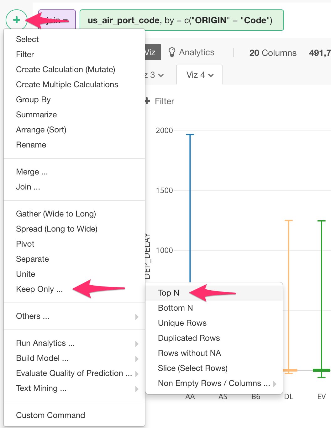
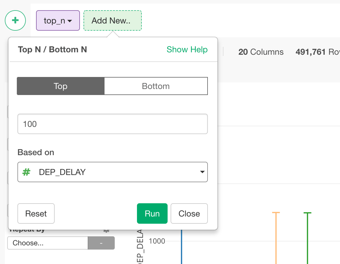
- Boxplot Chart with Grouped Top 100
- Scatter Chart with Trend Lines (Linear Regression Model and General Additive Model)
- Analyze Data with Machine Learning Algorithm
- Variable Importance with Random Forest
- Share Charts in Reproducible Way
- Create Note to Share insights
Download Flight Delay sample data
In this tutorial, we’re going to use US flight delay data for August, 2016, which tracks all the domestic flights that flew in the month for:- How much they were late or early for the departure / arrival delay times.
- Where they left from and arrive at.
- How long or far they were flying for each flight trip.
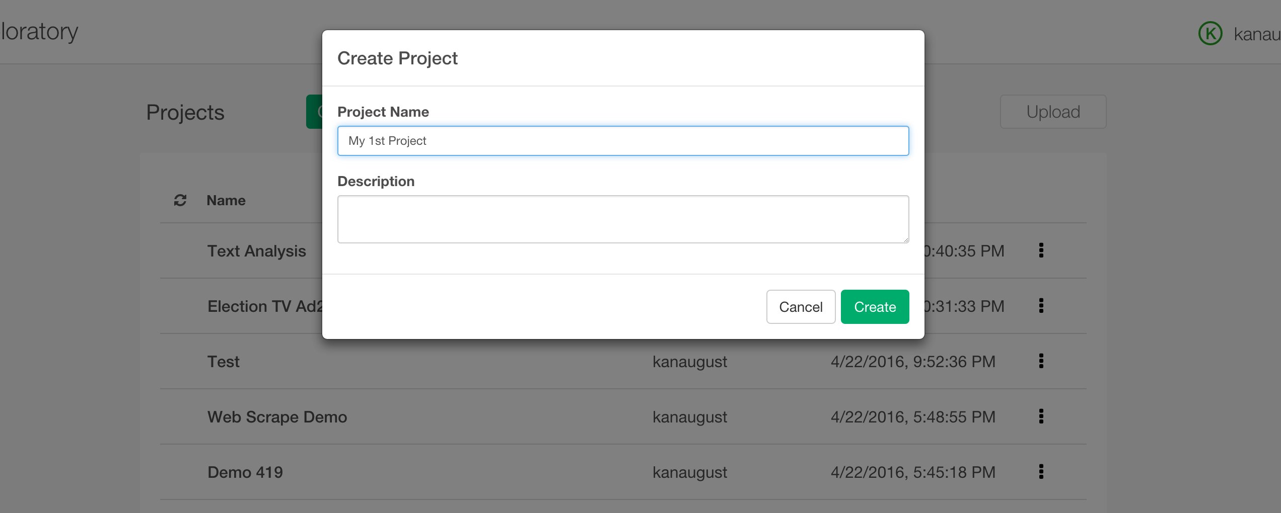
Create a new project
Once you start Exploratory app, create a new project to start.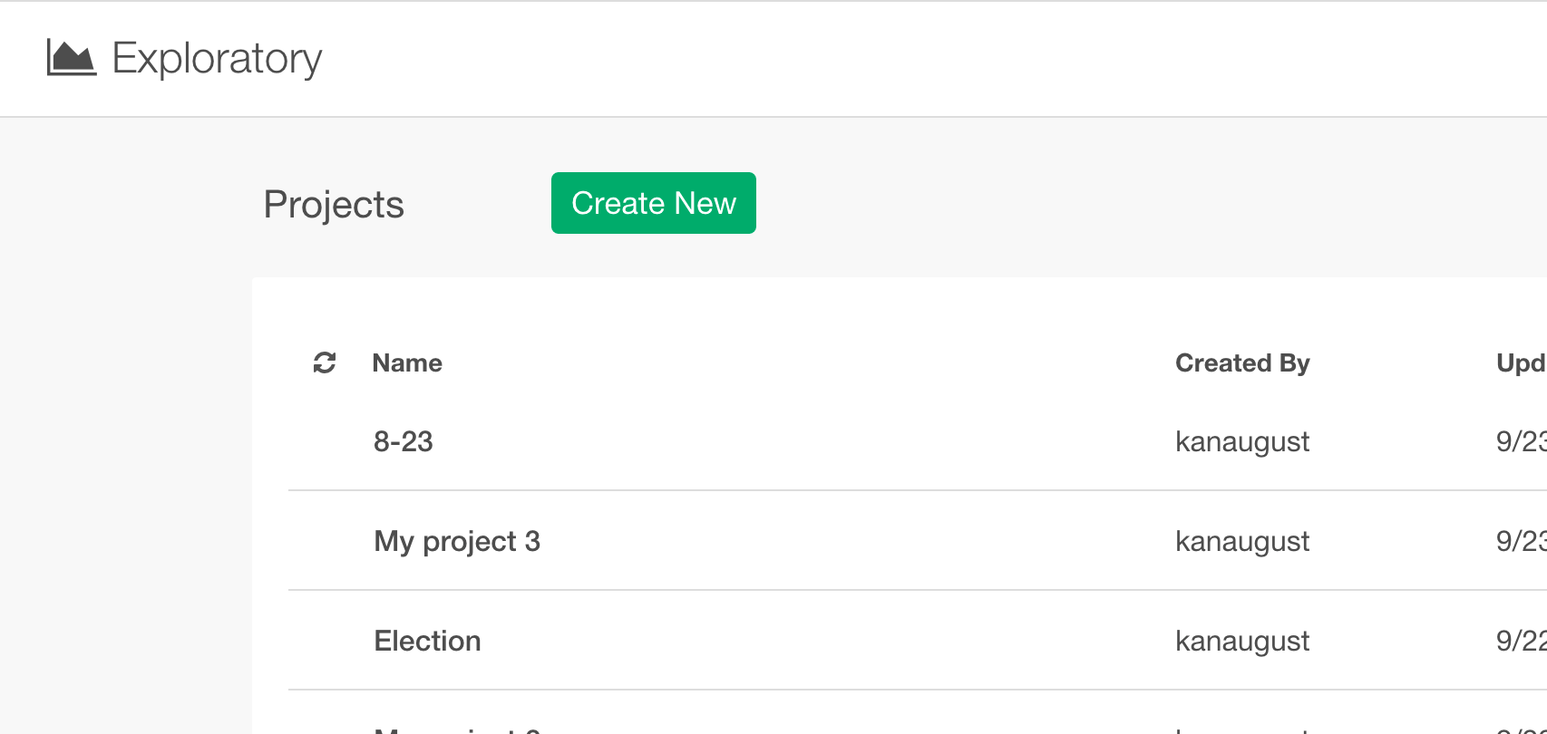
Import sample data
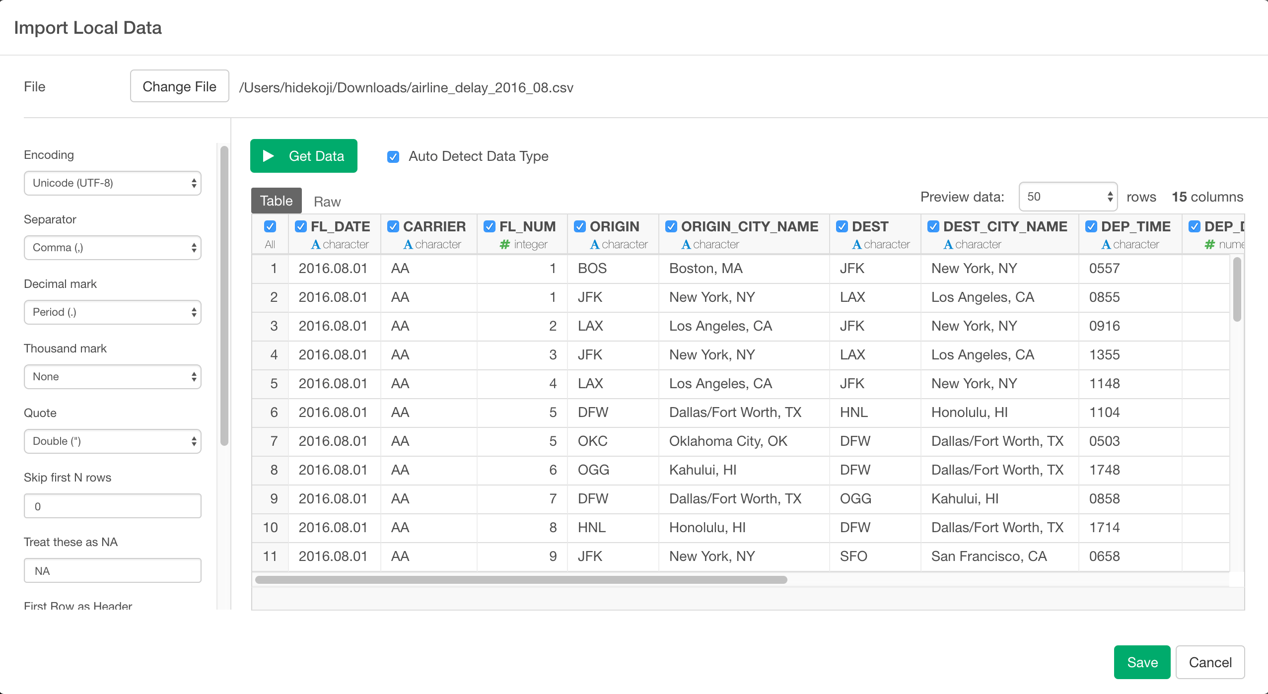
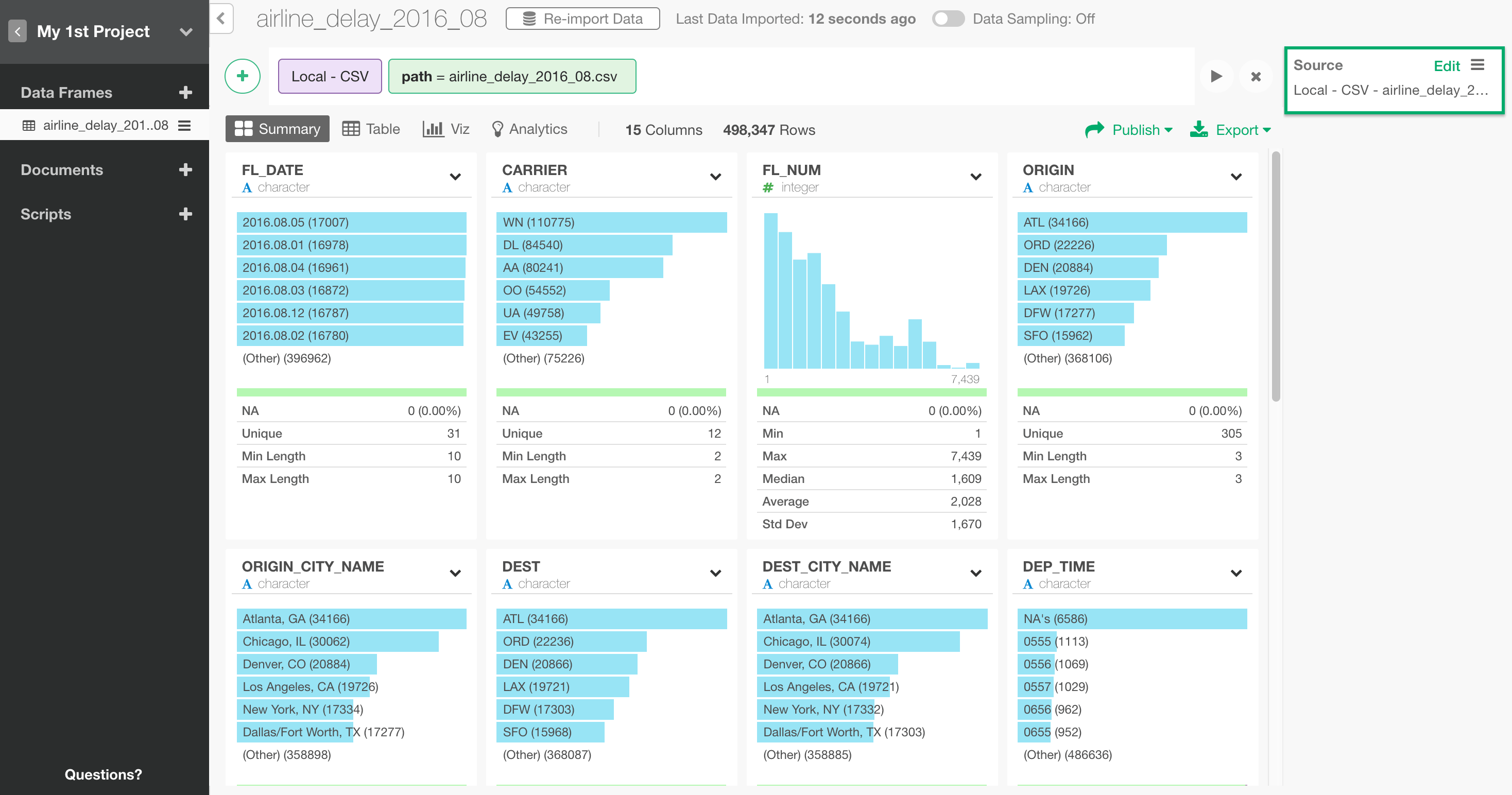
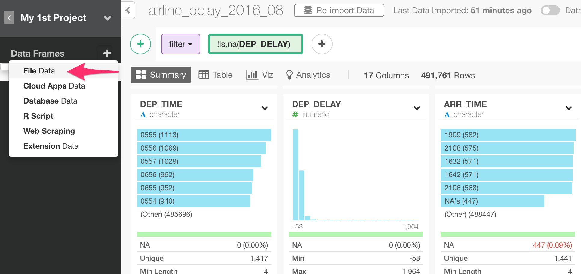
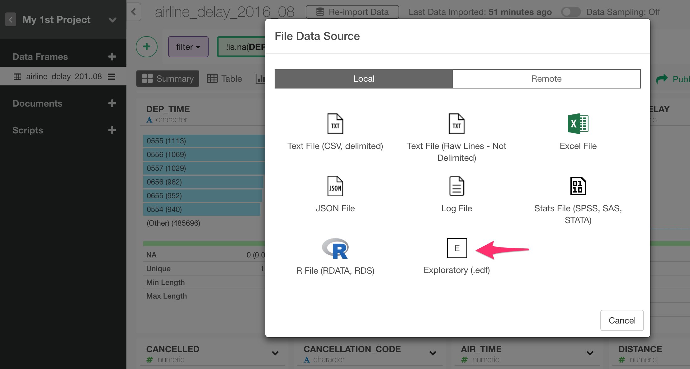
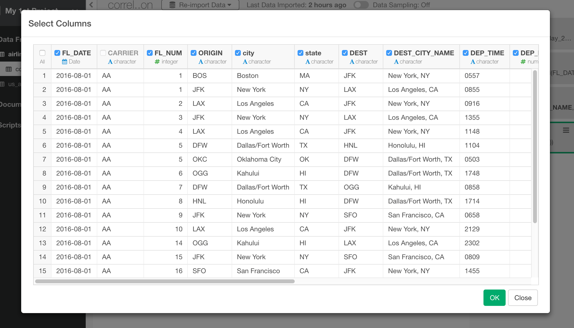
Inside the project, you can click on ’+’ (plus) button next to ‘Data Frame’ text in the left side pane, and select ‘Import File Data’ from the dropdown list.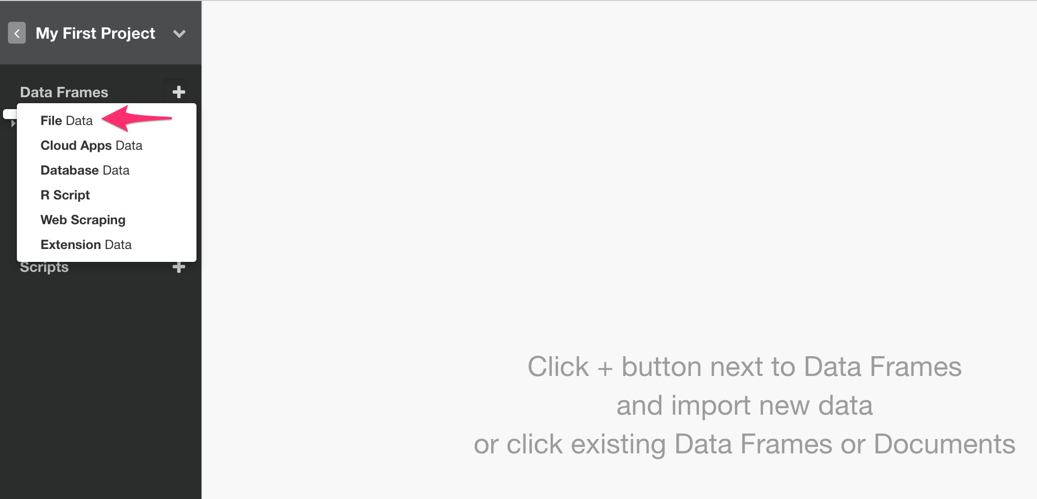
Inspect Data with Summary View
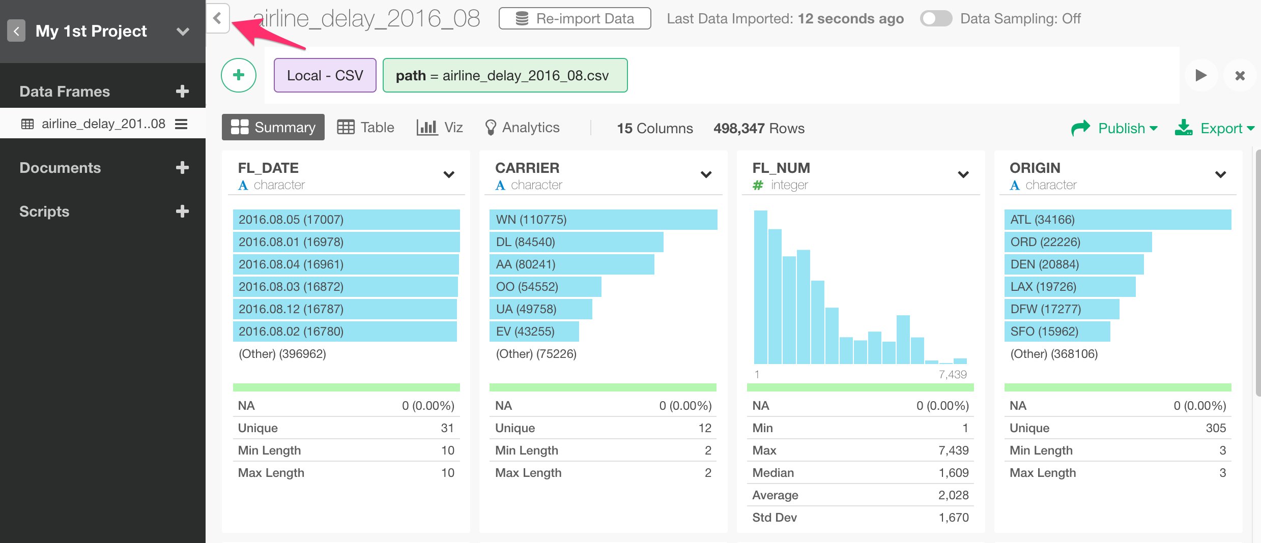
You can click ‘Summary’ tab and quickly see the summary information of the data in Summary view. For example, you can see that there are 12 unique airline carriers in CARRIER column and seven of them are listed as bar chart from the highest to the lowest.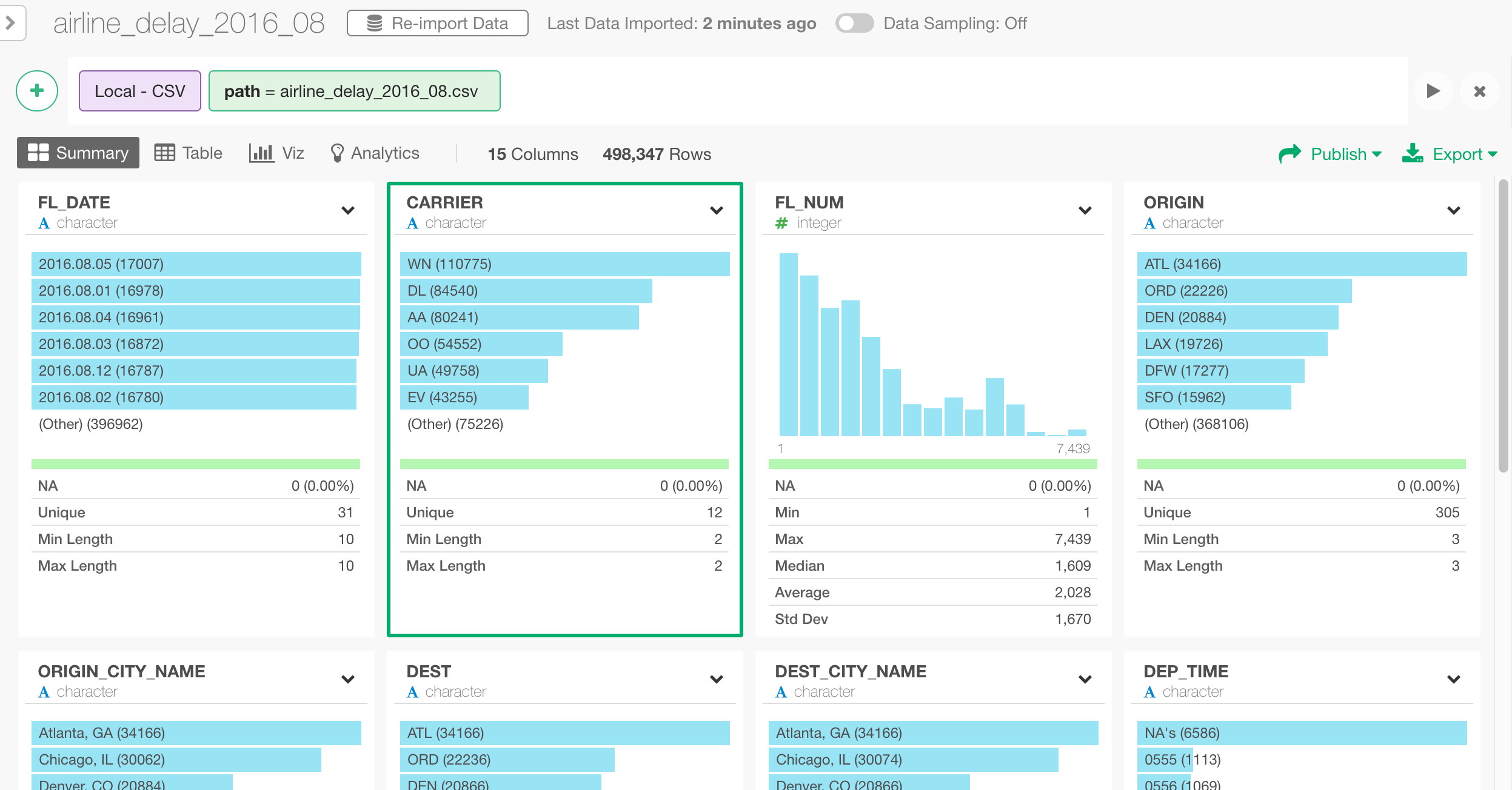
Transform Data (Data Wrangling)
In this Data Wrangling section, we are going to cover the following common data transformation tasks:- Parse character data and convert to Date
- Extract Day of Week information from Date
- Separate a column into multiple columns
- Remove NA (Missing Values)
- Join with Airport Location Data Set
Parse Character data and Convert to Date
As you can see below, FL_DATE column seems to contain date data but it’s registered as ‘character’ data type.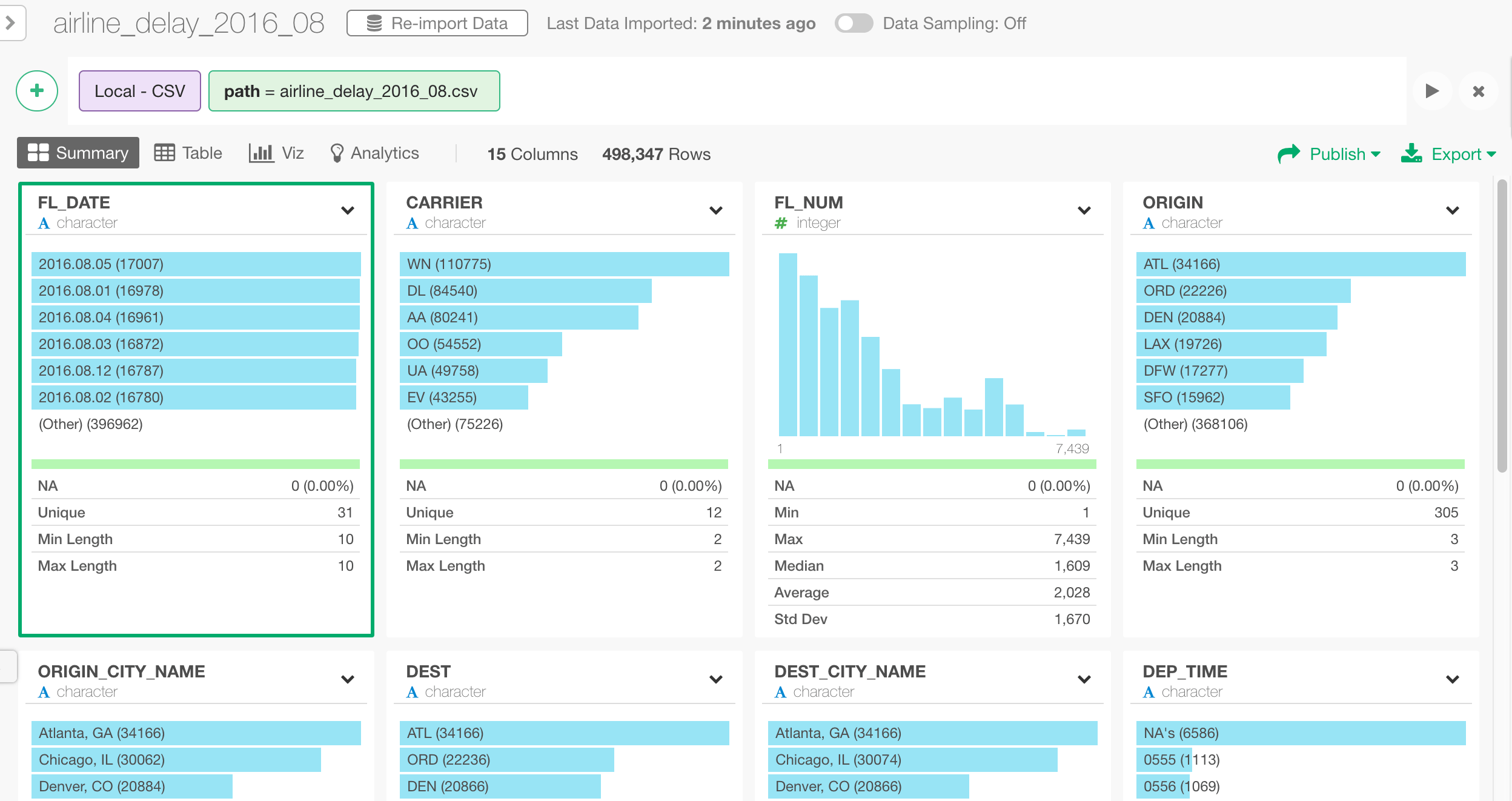
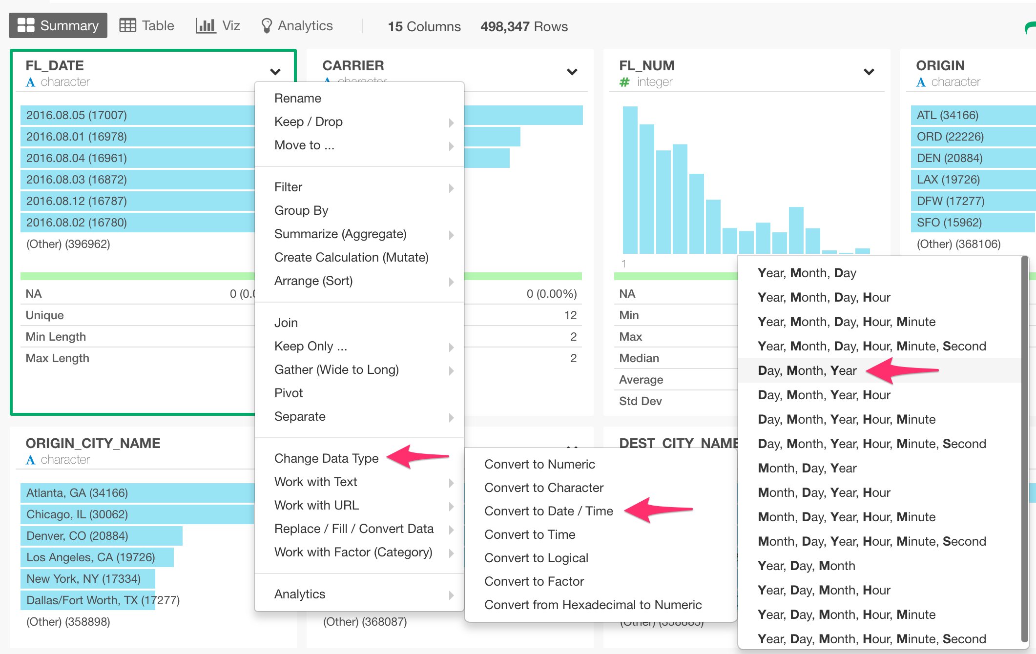
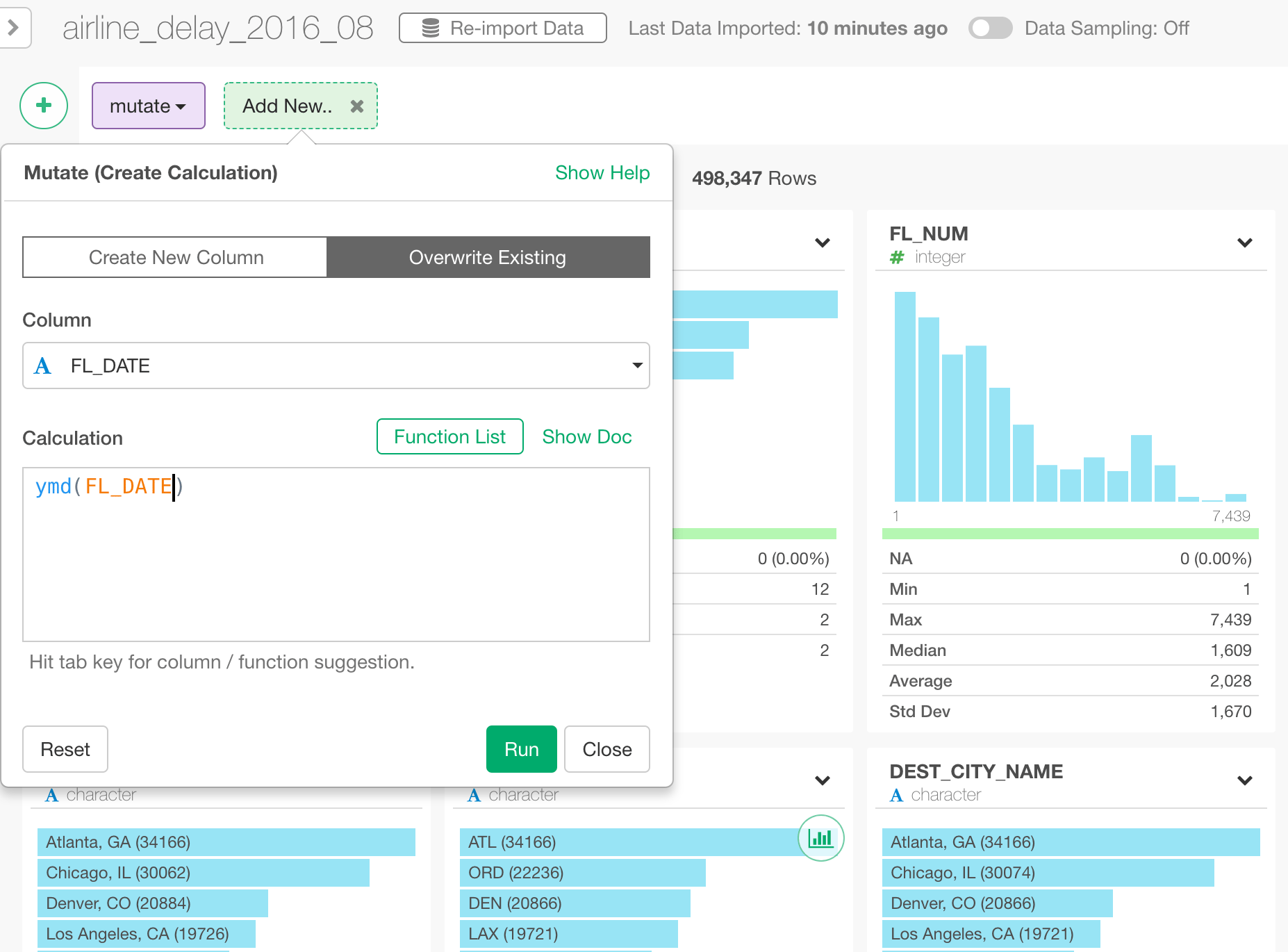
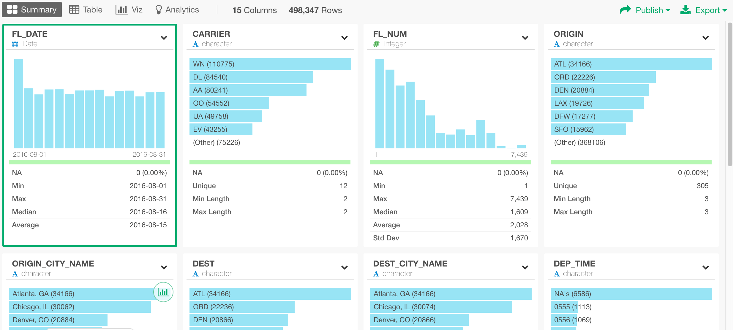
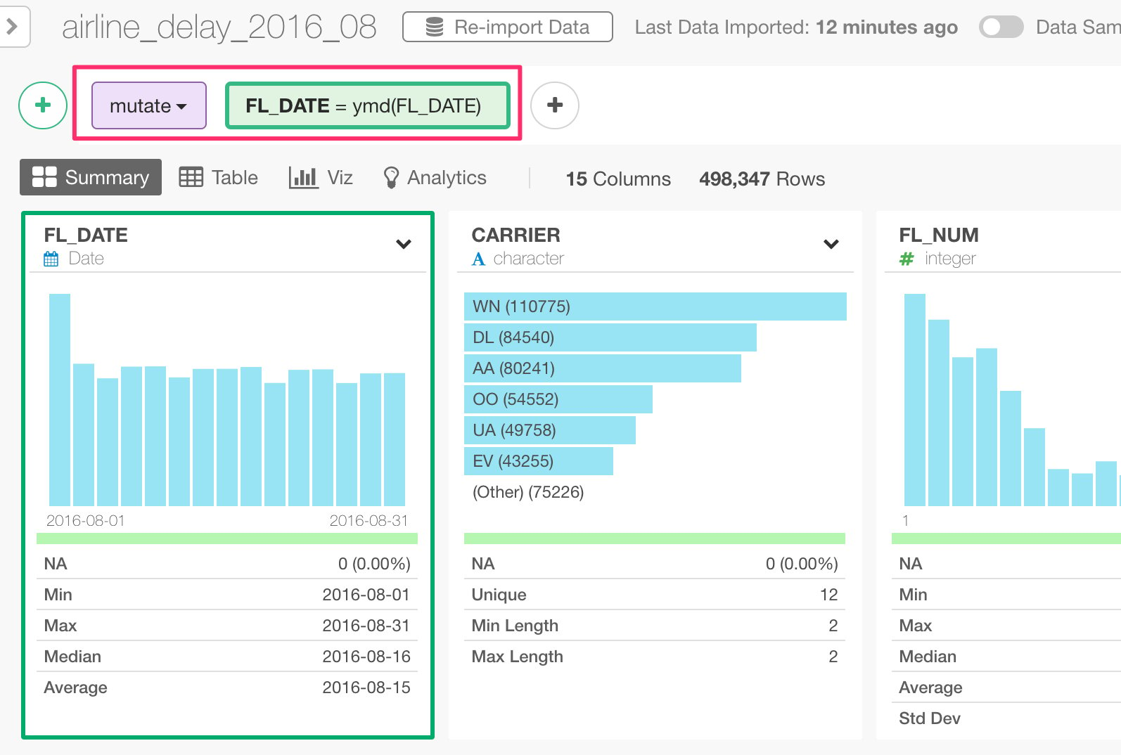
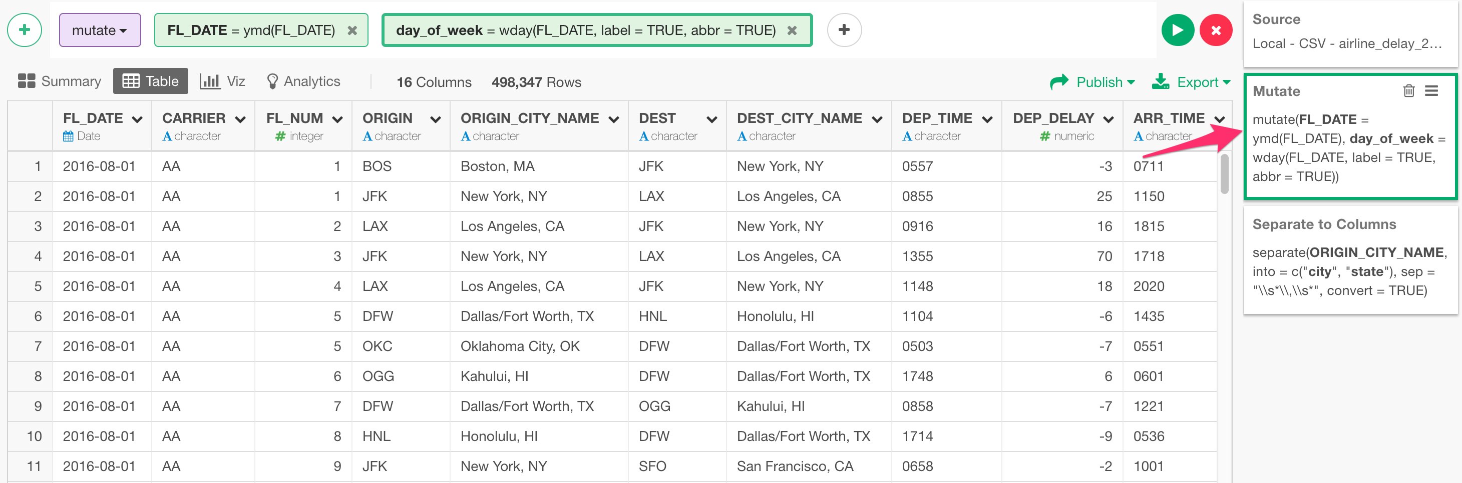
mutate. mutate command creates and runs new calculations, which is equivalent to Excel’s formula. You are going to see other types of the commands such as ‘select’, ‘summarize’, ‘filter’, etc. later, so no worry if you are puzzled here.
Now, in the green box you see the following.
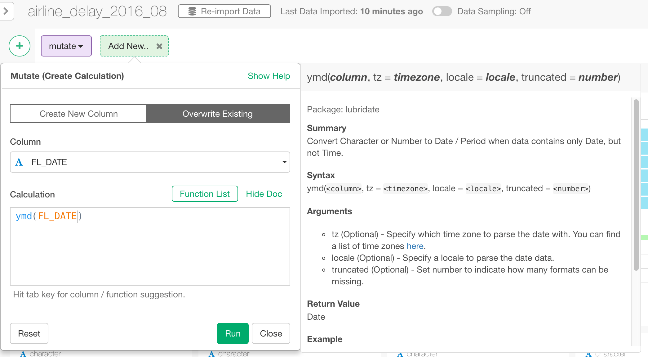
ymd() function, which you have seen previously.
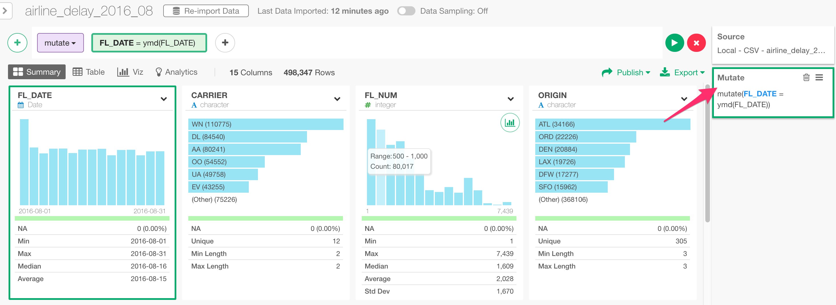
So basically, the ‘mutate’ command executes the calculation defined in the green box, in this case that is ymd(FL_DATE) and store the result into a column name called ‘FL_DATE’, which happens to be the original column name, so it will override the existing column values.
Lastly, you would also notice that there is a new step called ‘Mutate’ being added at the right hand side.
Extract ‘Day of Week Name’ from Date
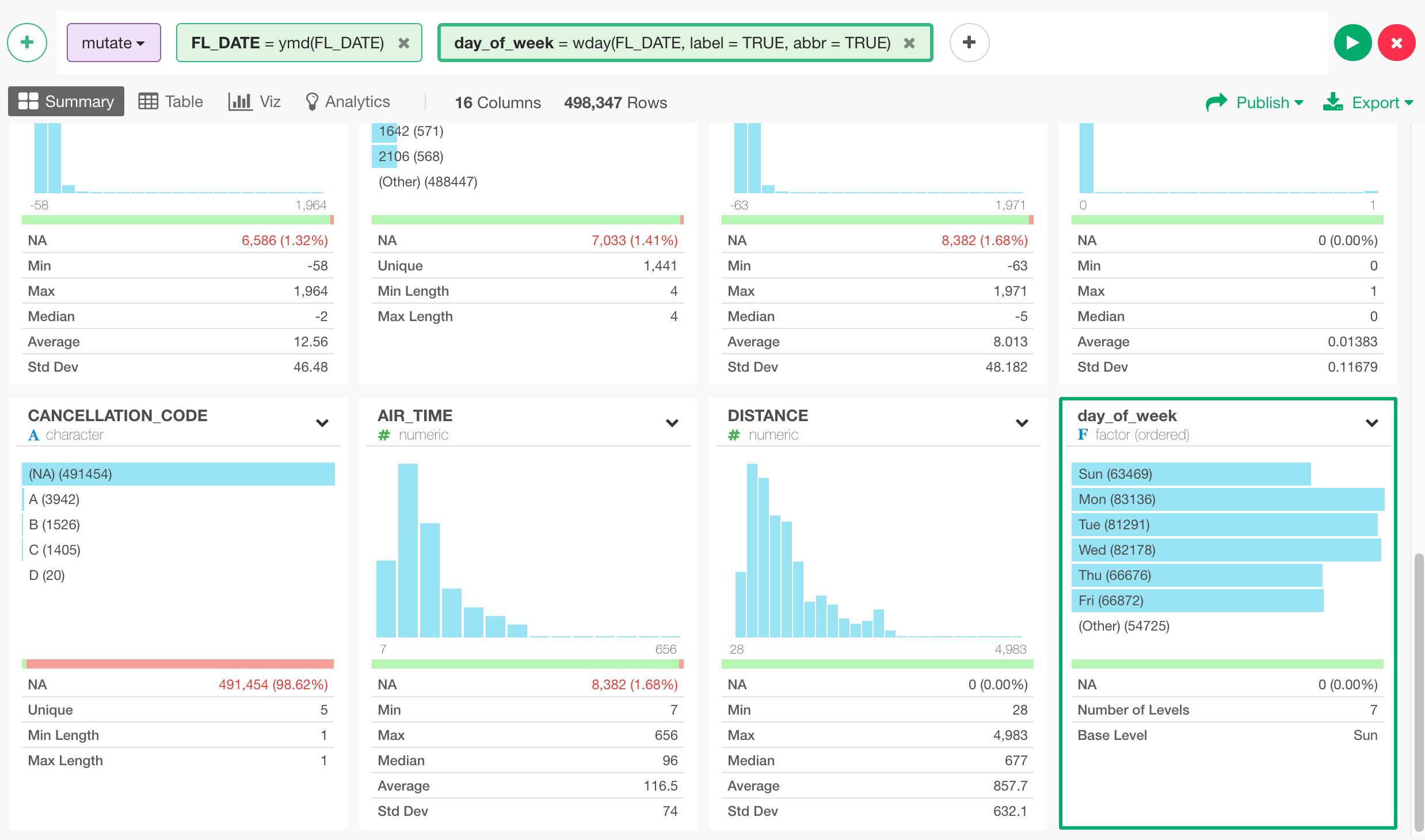
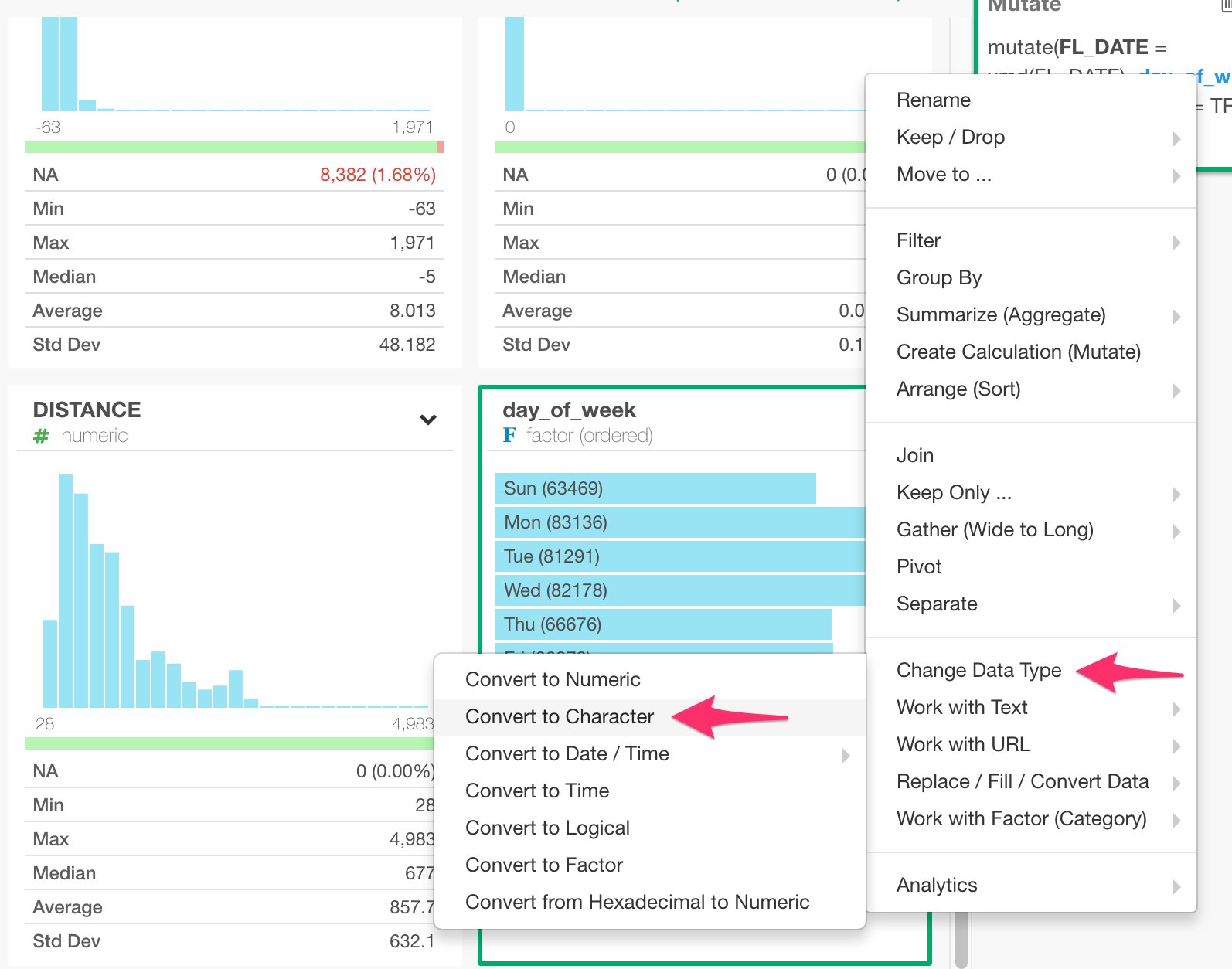
Let’s do one more operation within the same ‘Mutate’ step. Now that FL_DATE column is ‘Date’ data type, we can extract date component information like ‘Day of Week Name (e.g. Sun, Mon, etc.)’. You can select ‘Extract’ -> ‘Day of Week Name (e.g Mon)’ from the column header menu.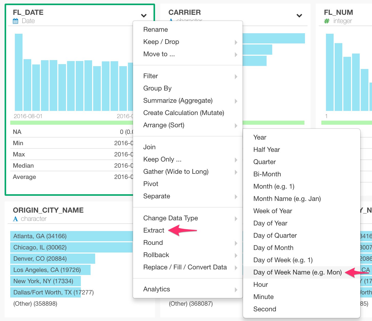
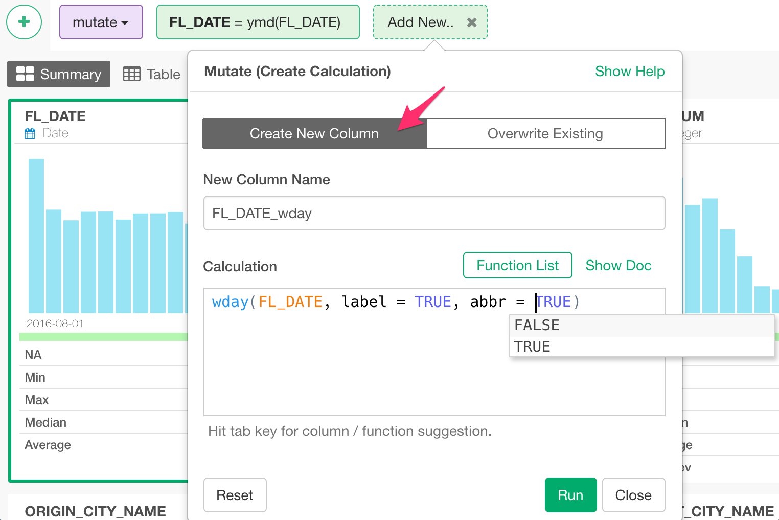
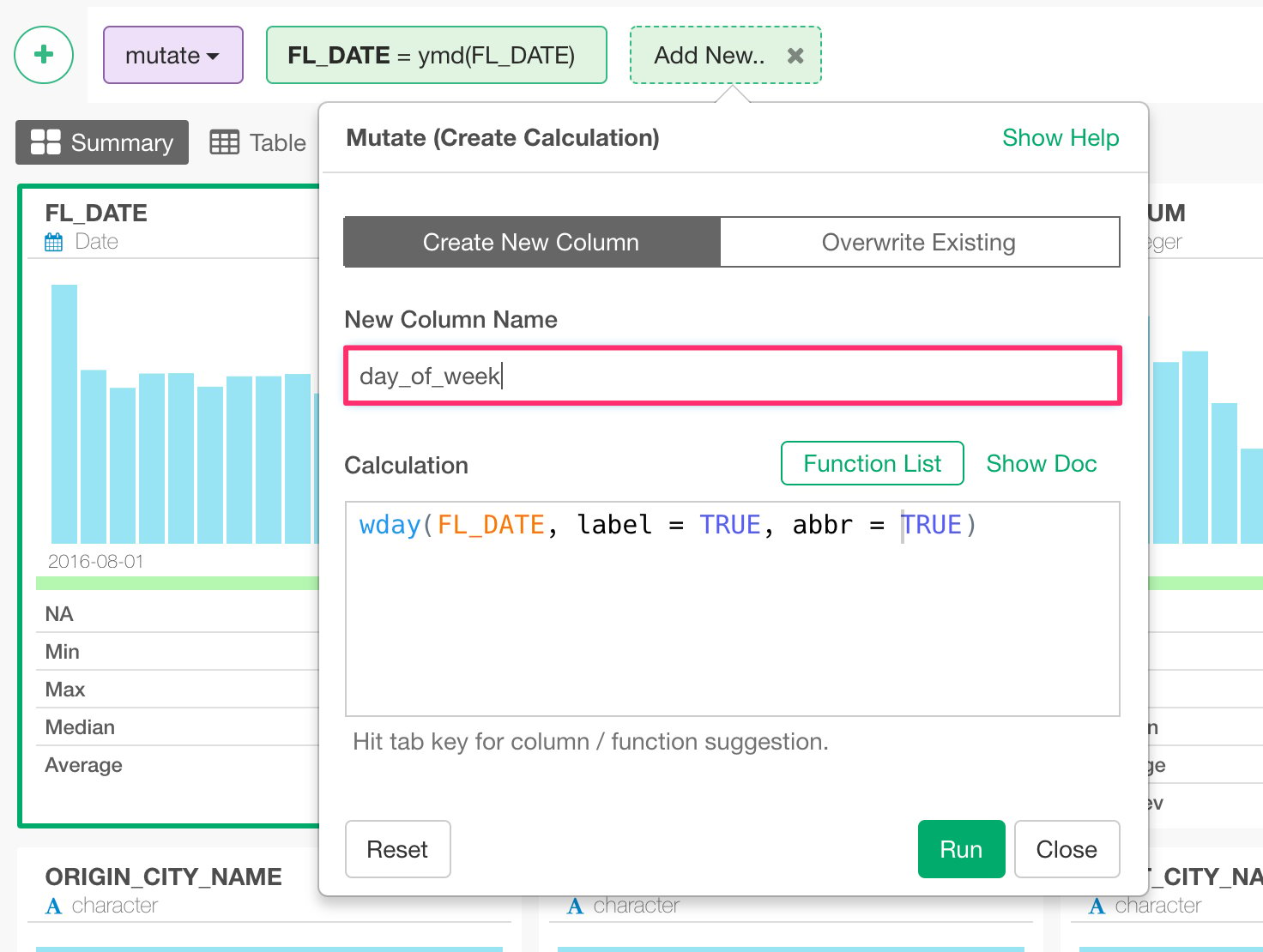
wday(FL_DATE, label = TRUE, abbr = TRUE), instead of overriding the original column like the last time.
Type ‘day_of_week’ for the new column name, and hit ‘Run’ button.
Separate a column into multiple columns
Let’s take a look at how you can separate a column into multiple columns. Here, ORIGIN_CITY_NAME column contains both city names and US State names.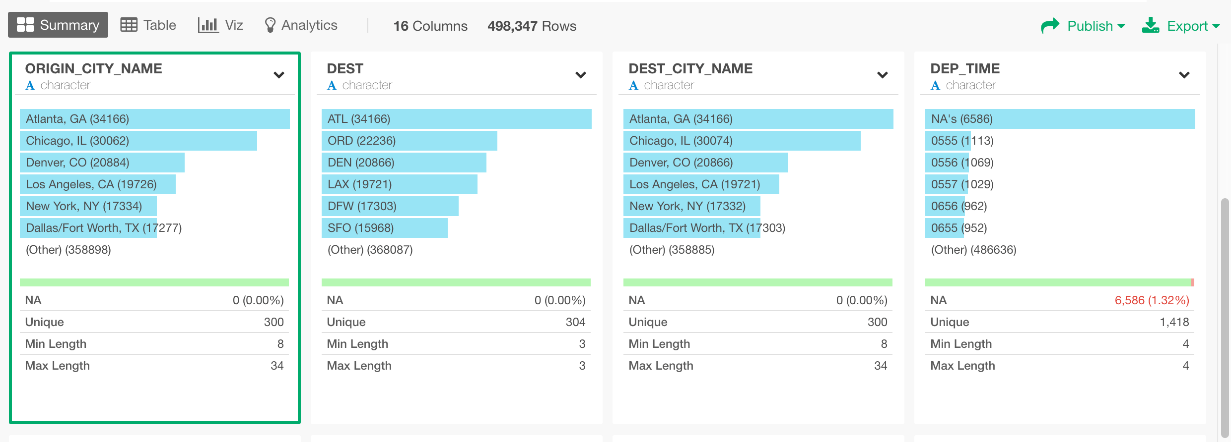
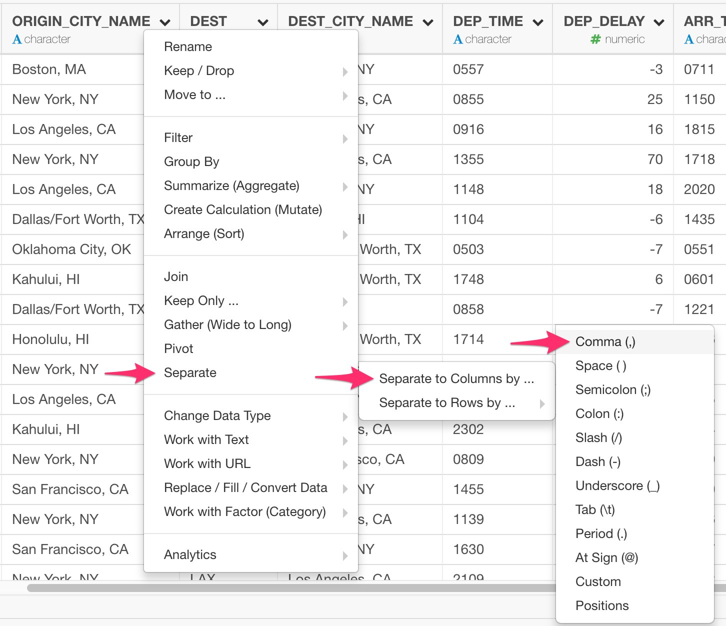
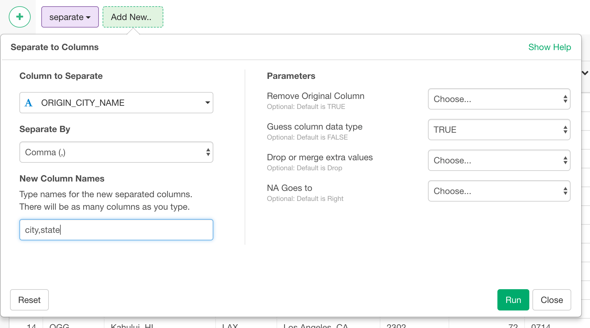
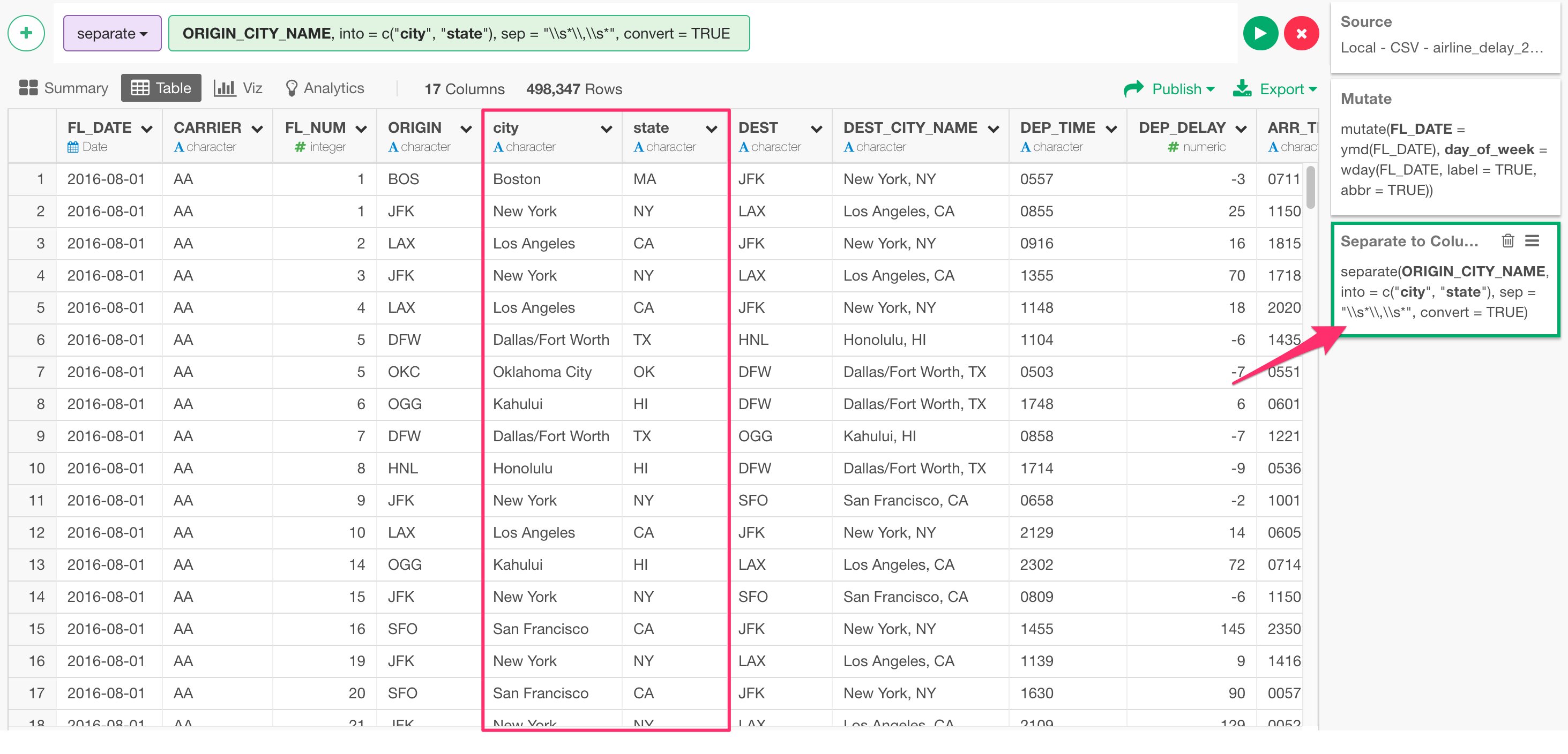
Work with NA (Missing Values)
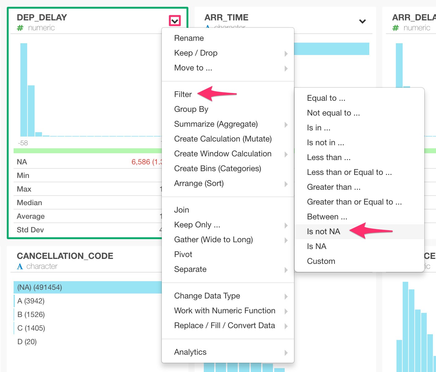
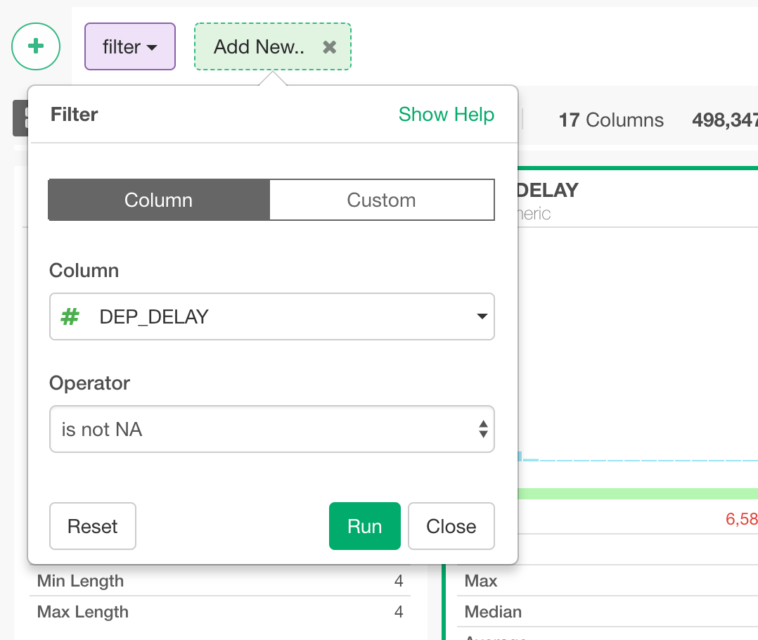
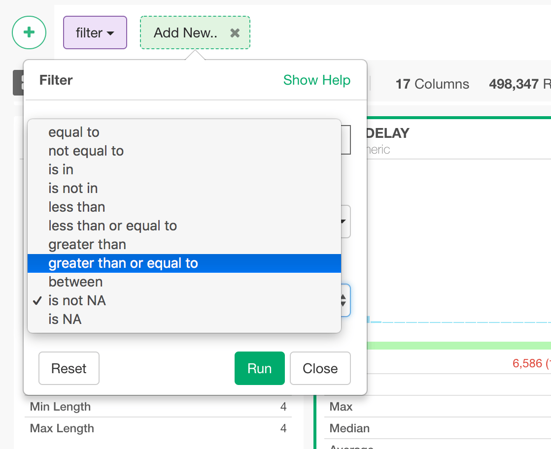
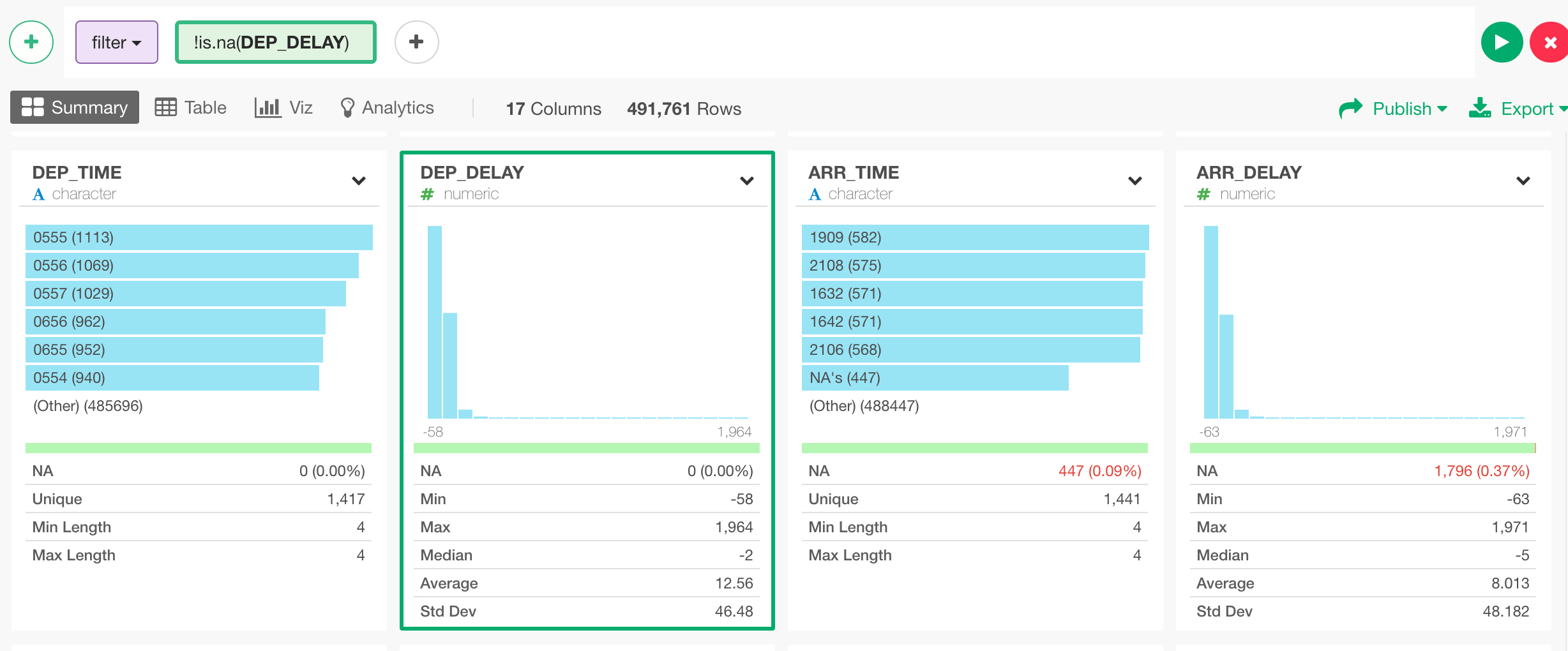
When you look at DEP_DELAY column in Summary view, you would notice that there is a slight red color in the green bar.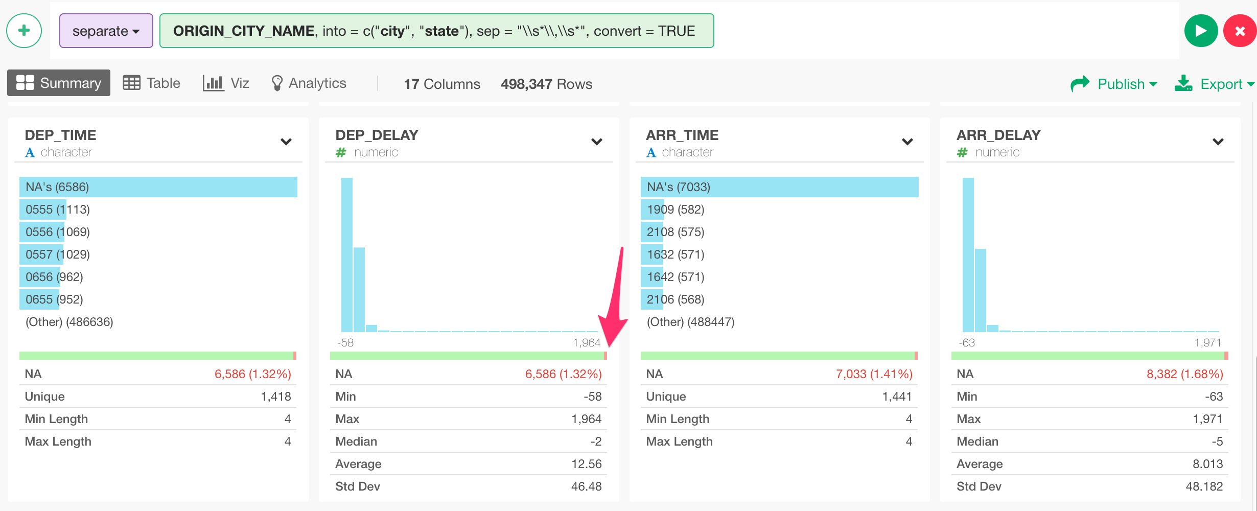
Join with Airport Location Data Set
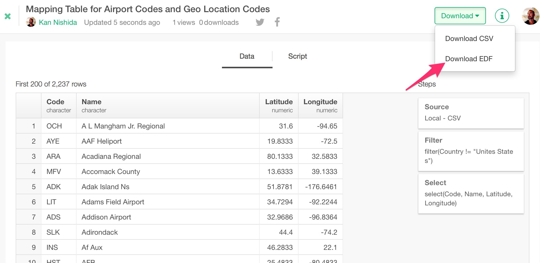
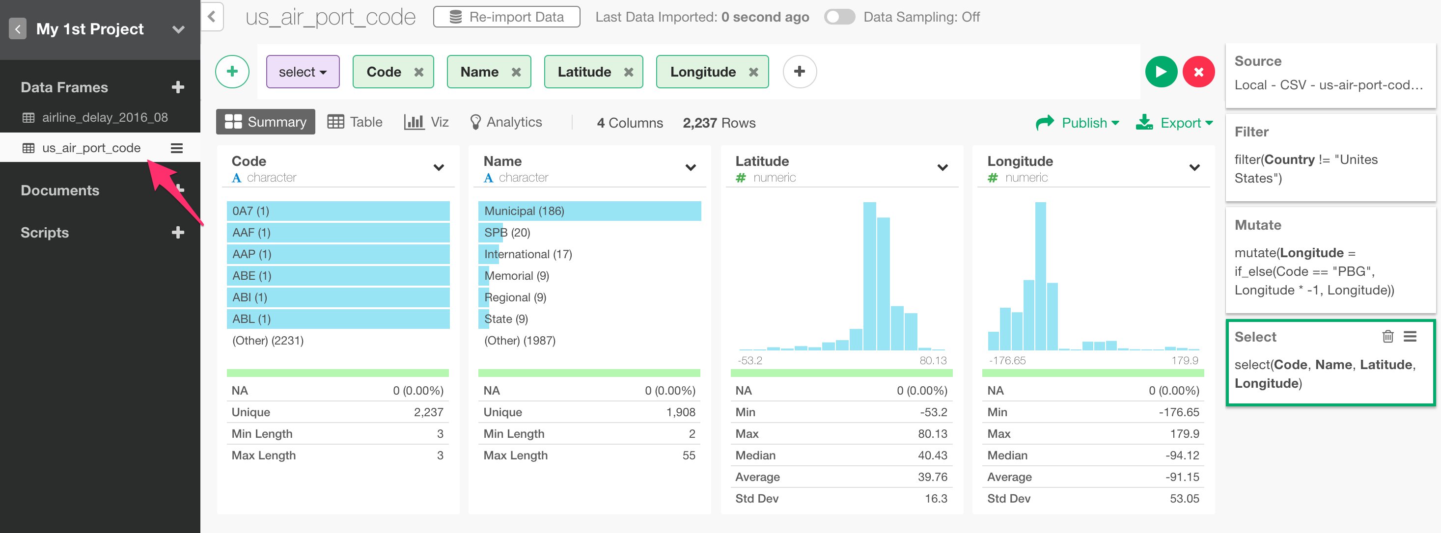
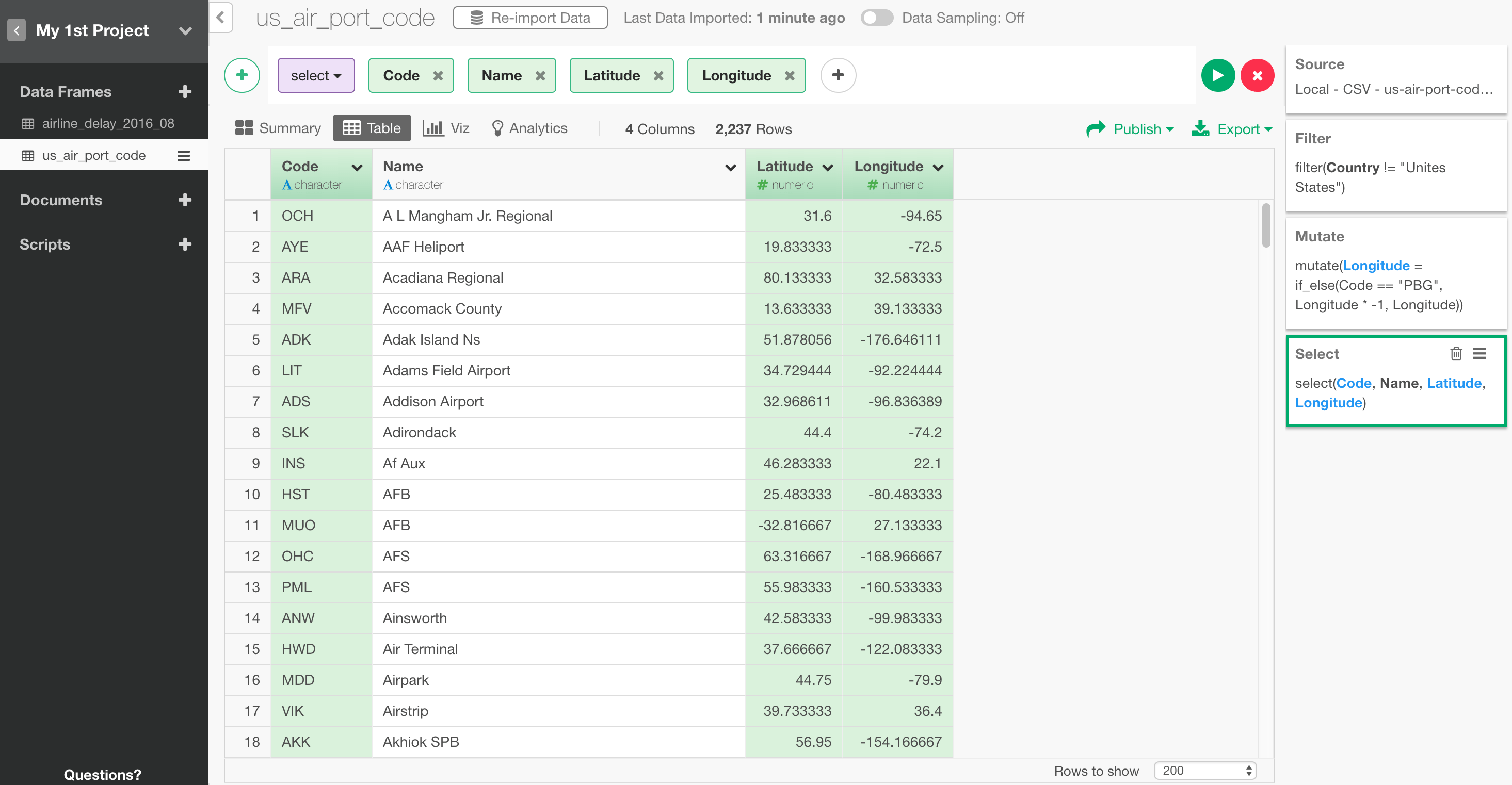
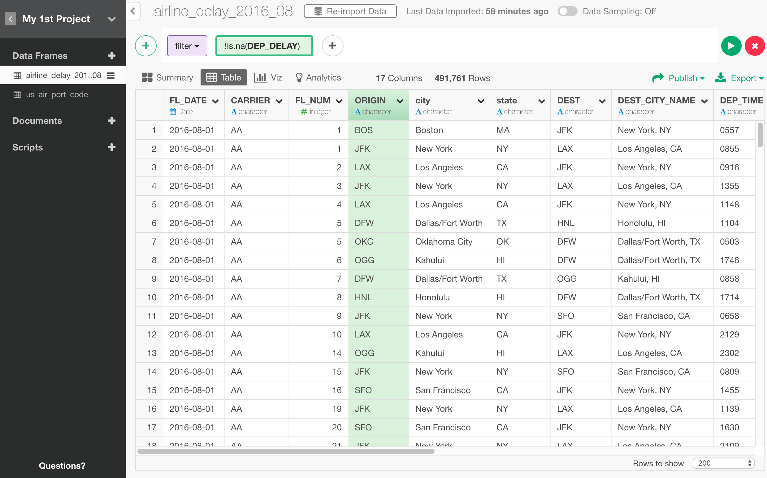
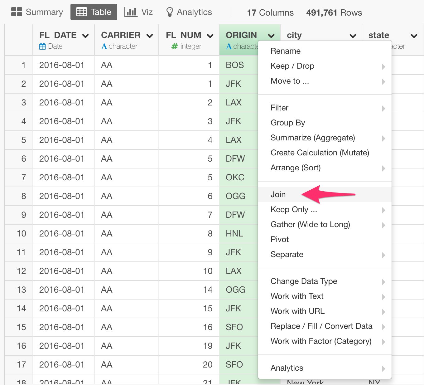
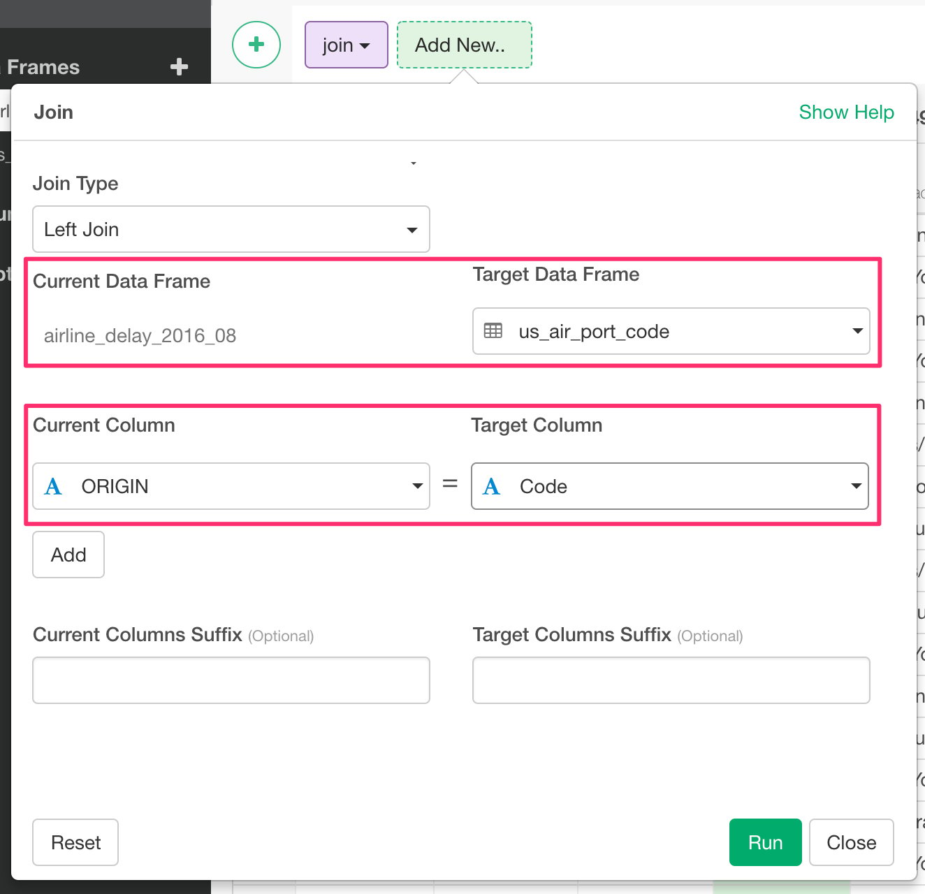
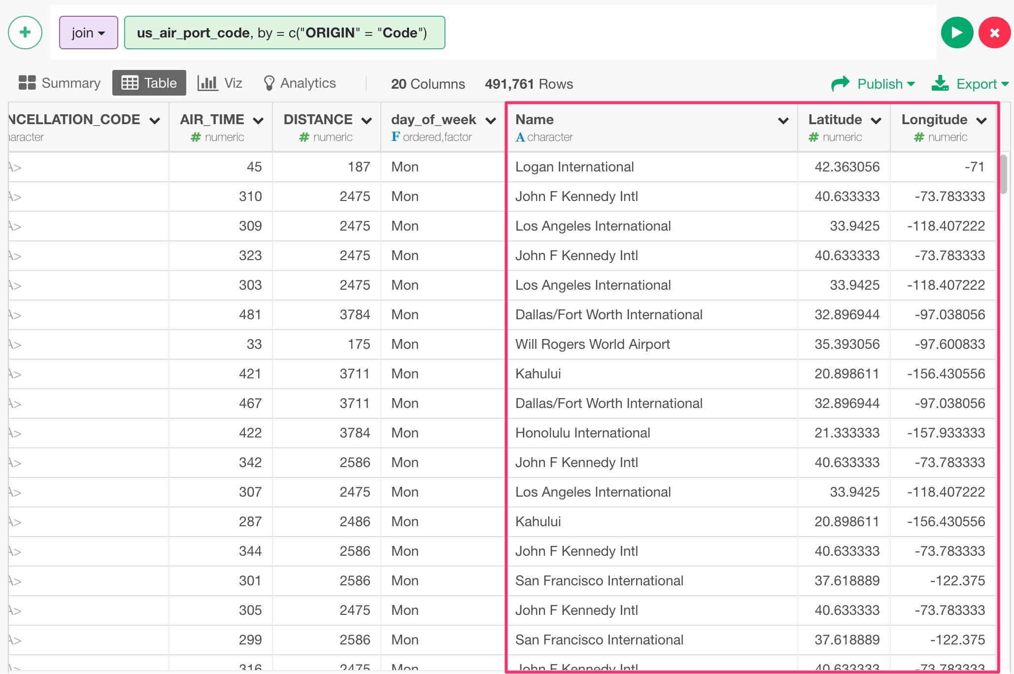
Let’s say we want to visualize where these airports are located on Map. We have airport codes in the data, but there is no geo location codes (longitude and latitude) associated with the airports. So, what we can do here is, first, find a mapping table that maps between the airport codes and the geo location codes. You can find such mapping table easily on the web, but here is one we have published as EDF (Exploratory Data Format) file so that you can import to your Exploratory in a reproducible way. Once you download and import it into your Exploratory, then we can use this mapping table data to assign the geo location codes for each airport code in the ‘airline_delay_2016-08’ data frame. Basically, it’s similar to what you would do with ‘vlookup’ in Excel or with ‘join’ operation in SQL or typical BI tools. In Exploratory, you can use one of the ‘join’ commands called ‘left_join’, which would join two data frames by adding columns from ‘target’ data frame by matching ‘key’ column values from both data frames. It looks something like below.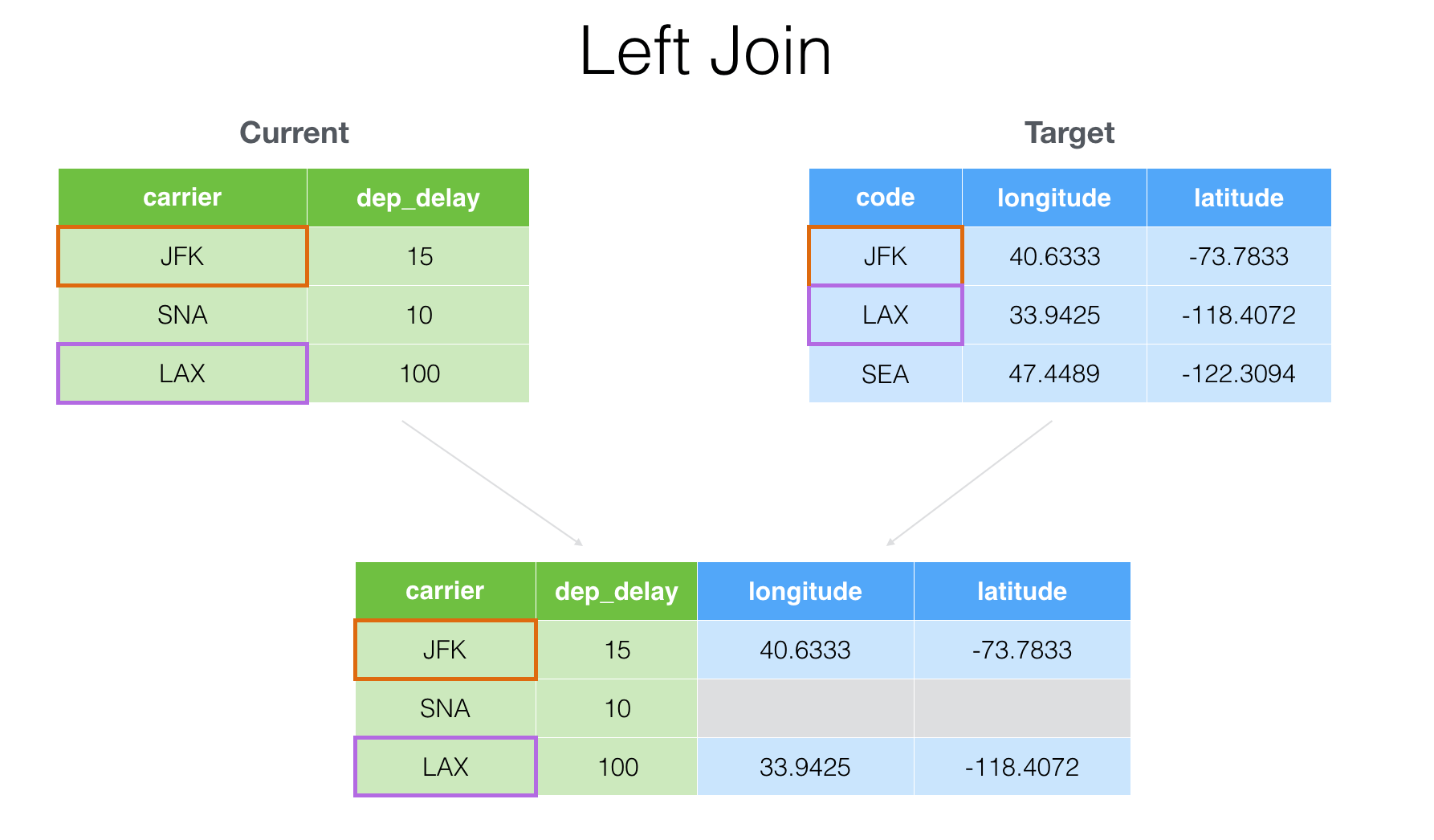
- Introduction to Join — Bring extra columns from the target in Exploratory
- Introduction to Join — filtering data based on the target data in Exploratory
Visualize data
There are many ways to visualize data with various chart types in Exploratory. In this exercise, let’s use the following chart types to explore the data.- Map - Understand where the flights are leaving from.
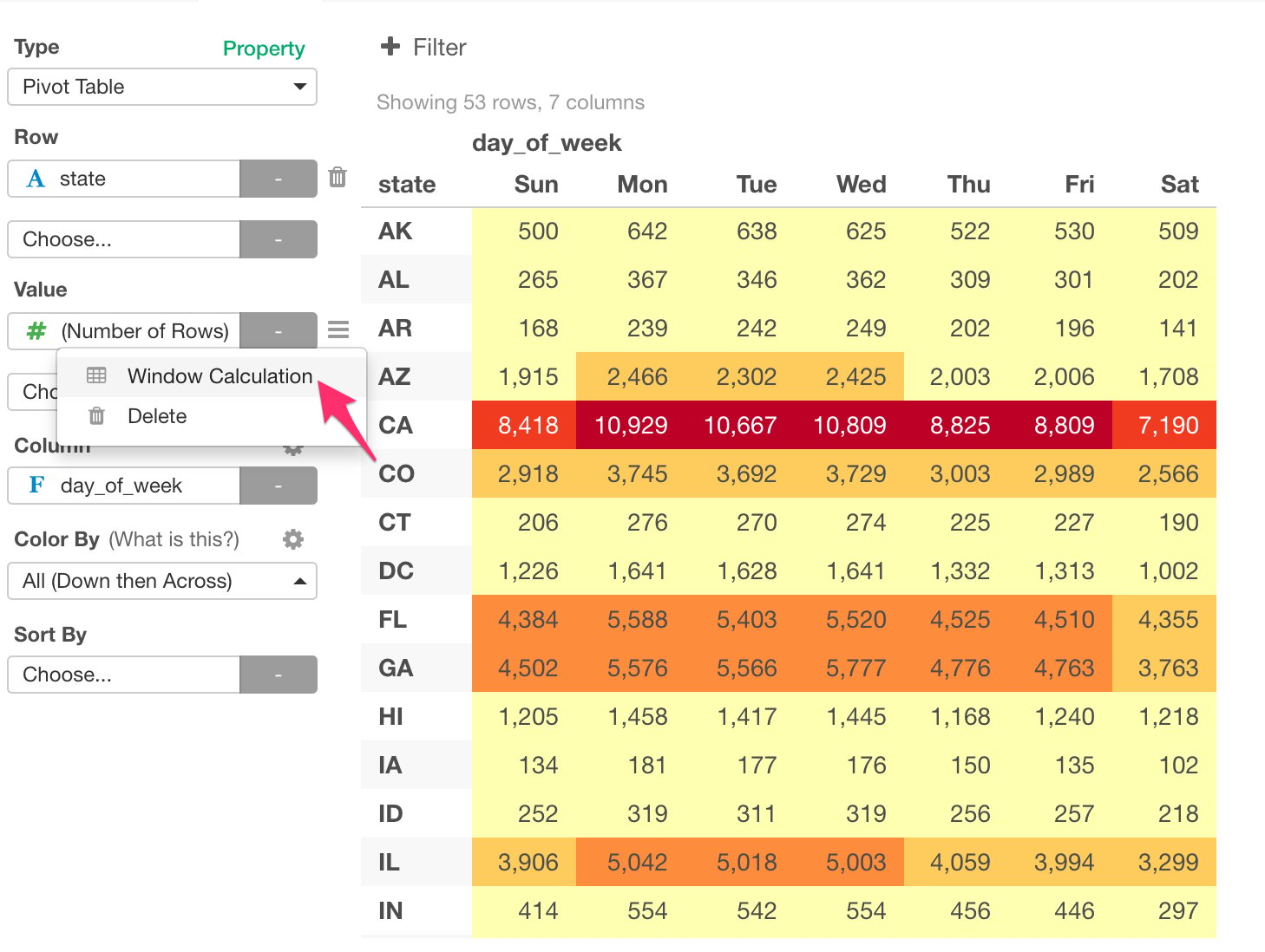
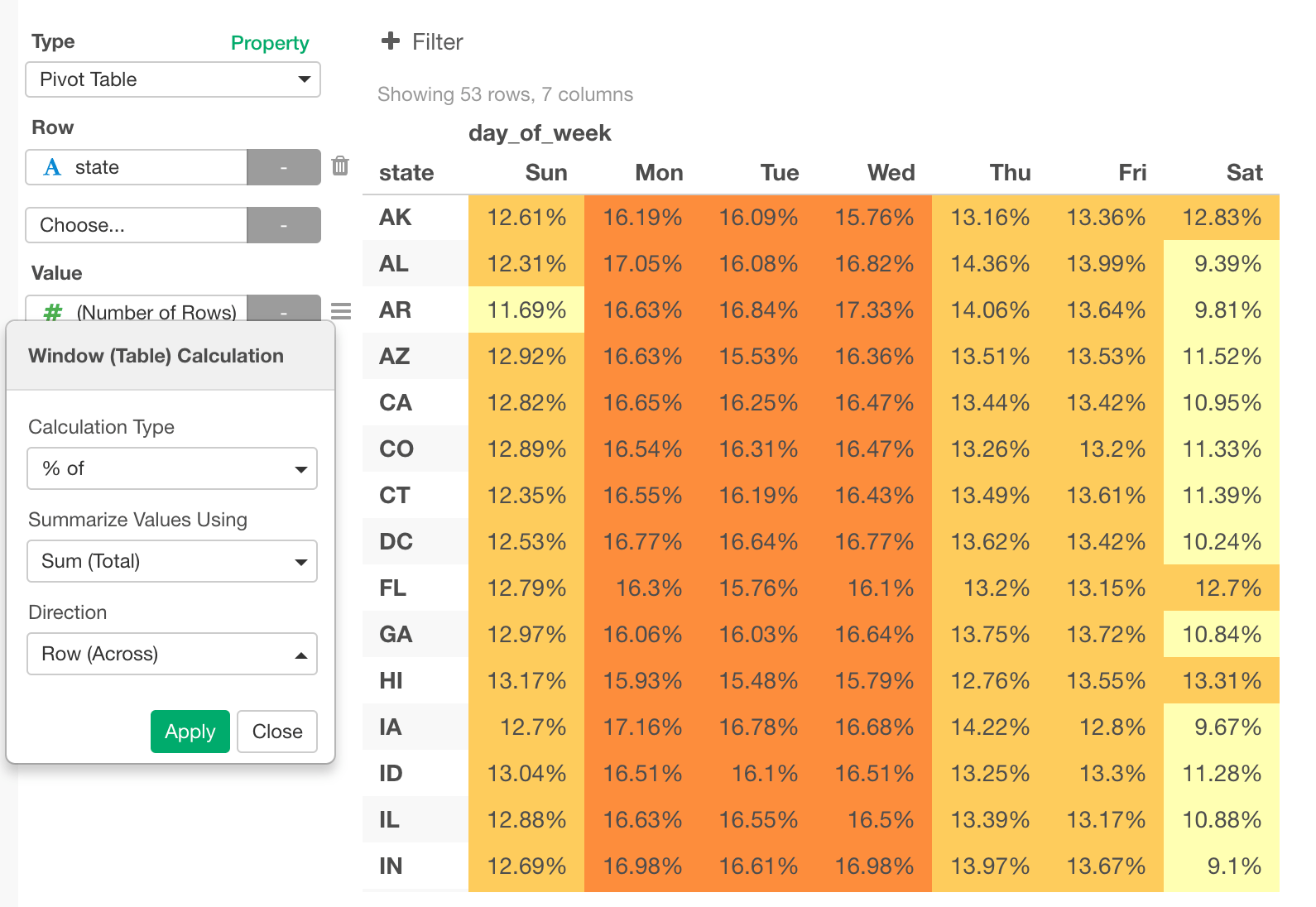
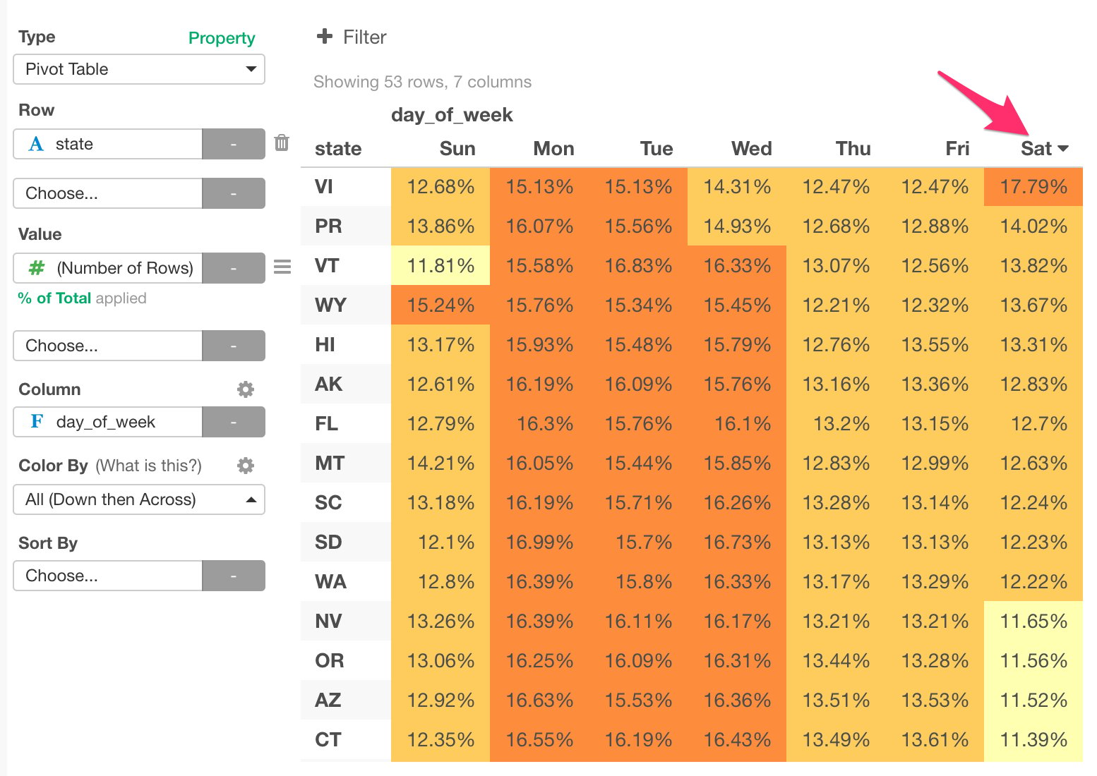
- Pivot Table - Understand which state and day pairs have more flights than the others.
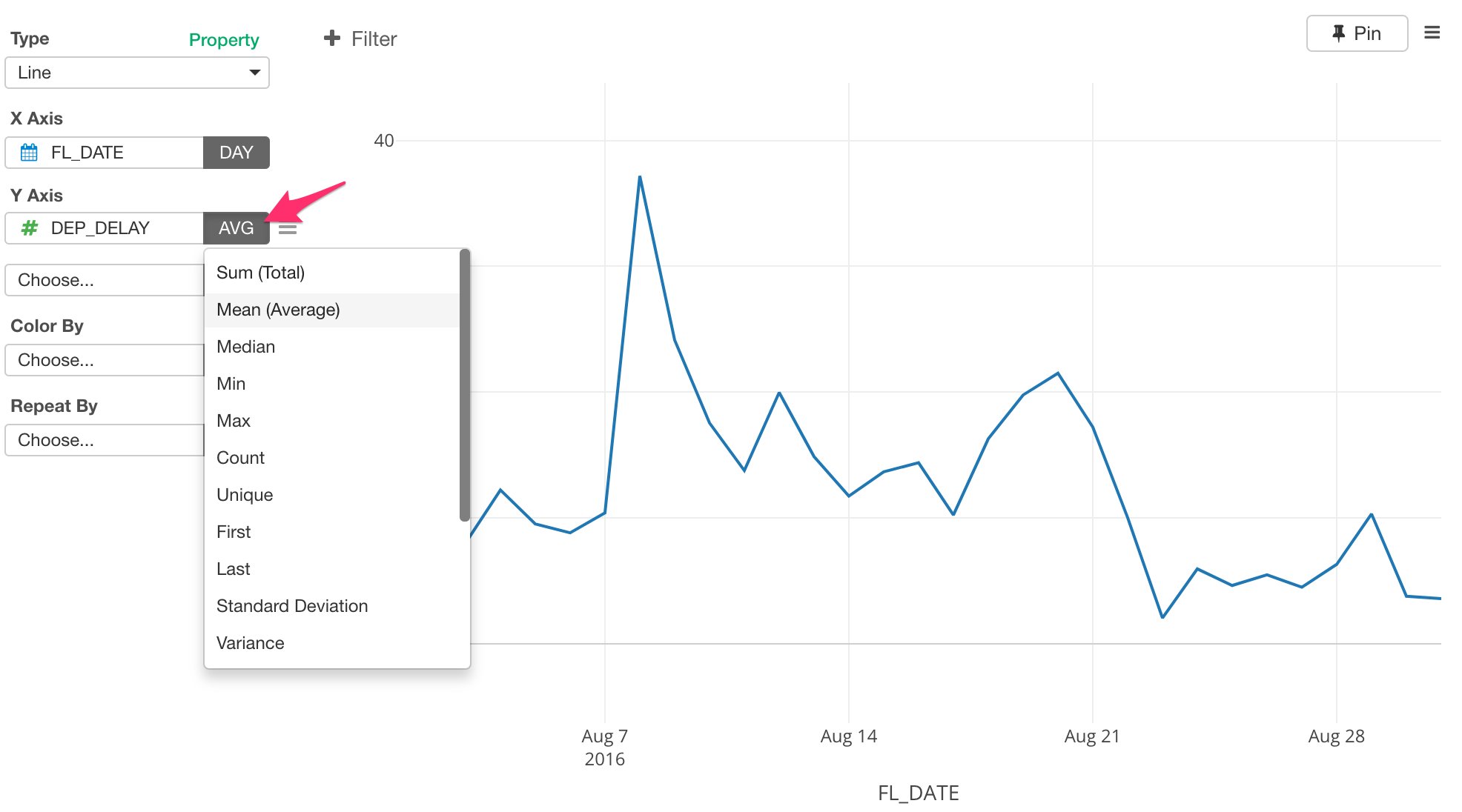
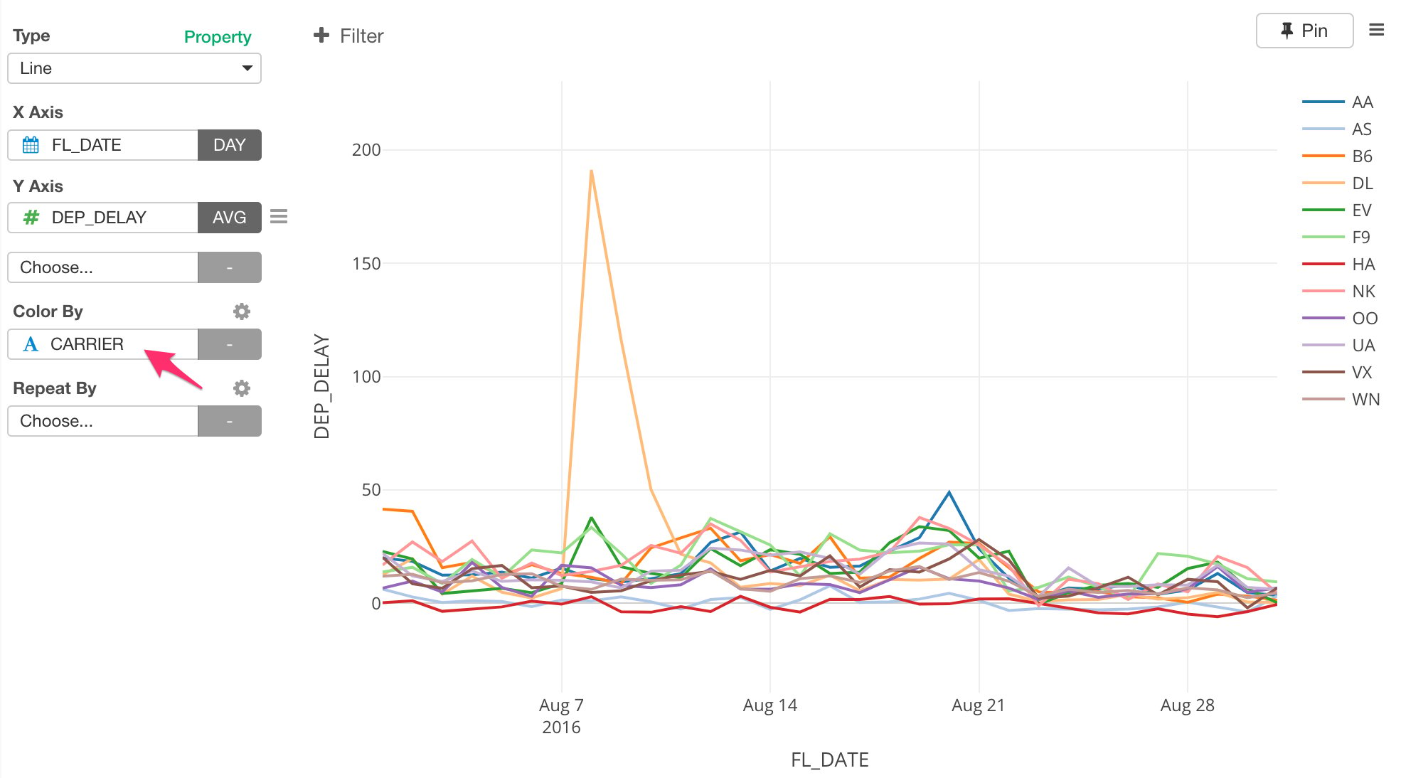
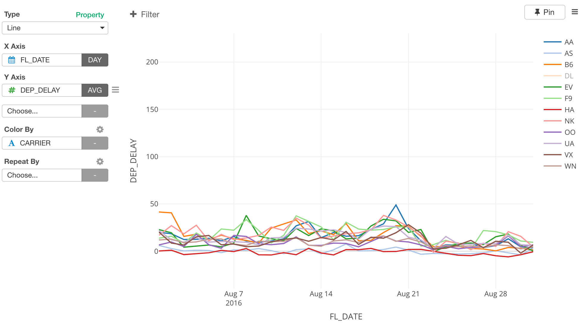
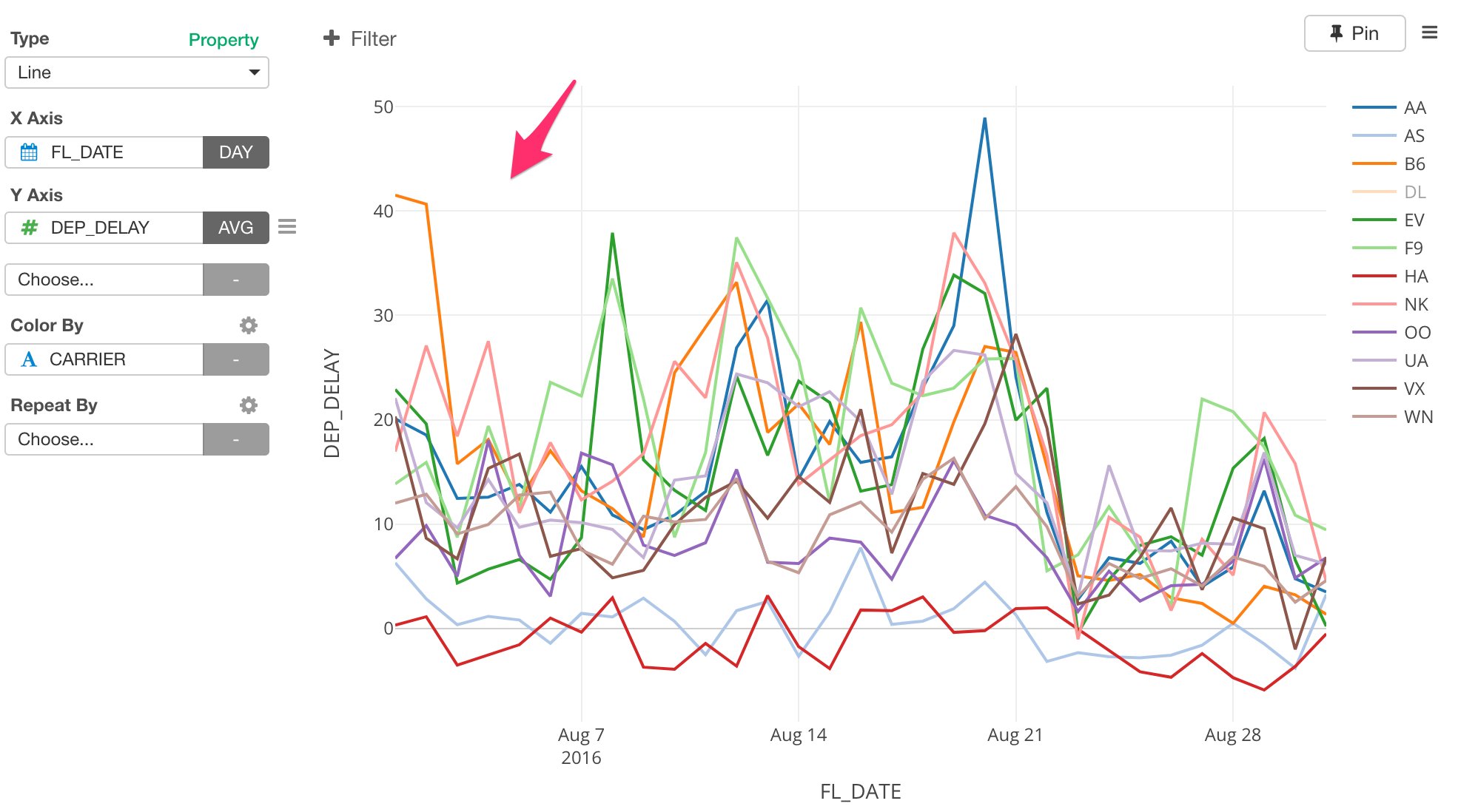
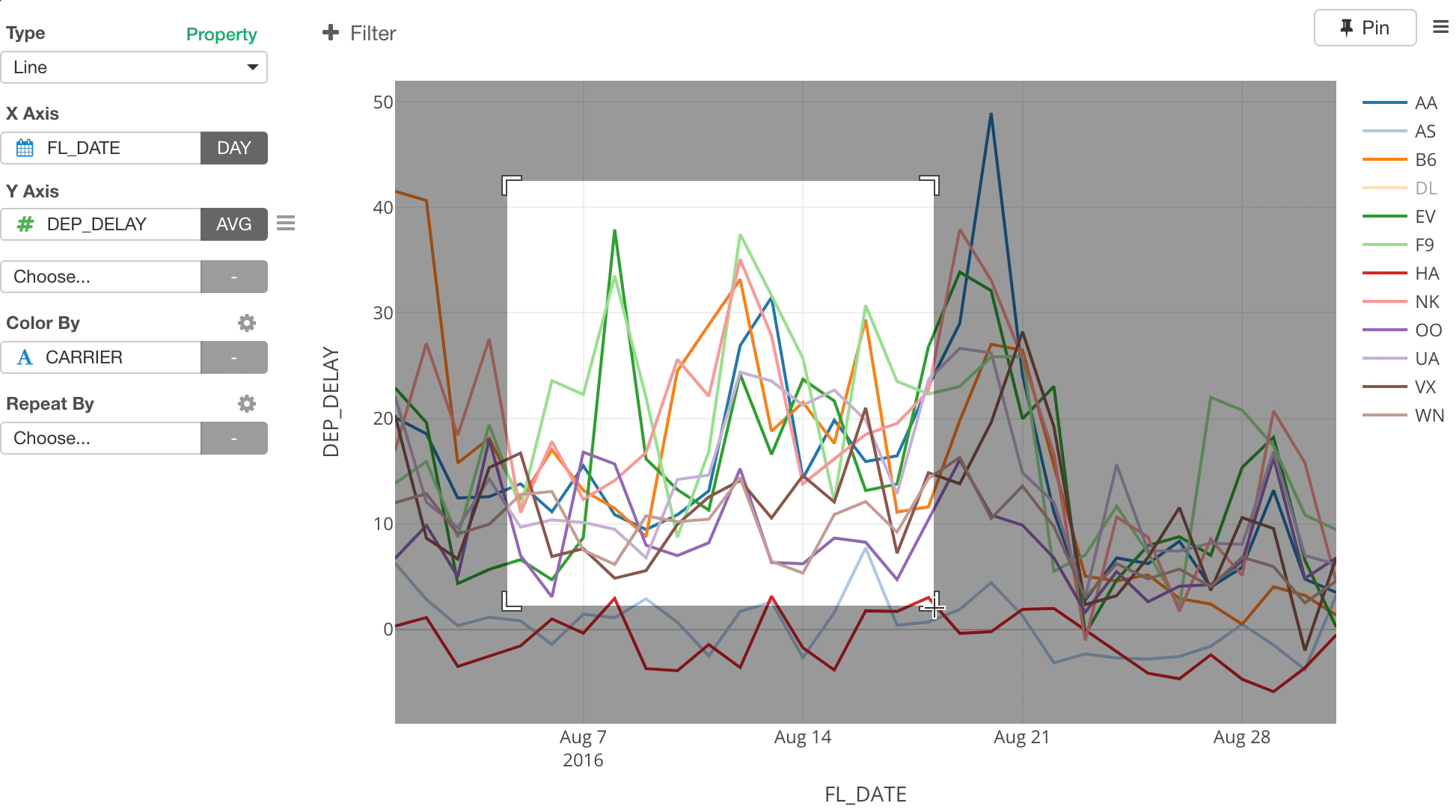
- Line Chart - Understand the trend of the departure delay times in August.
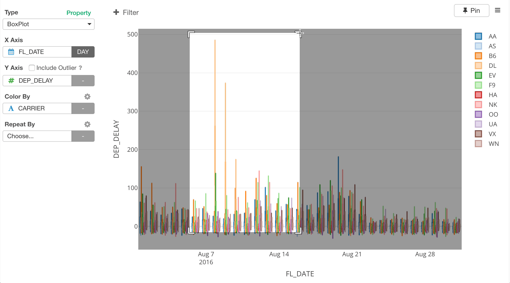
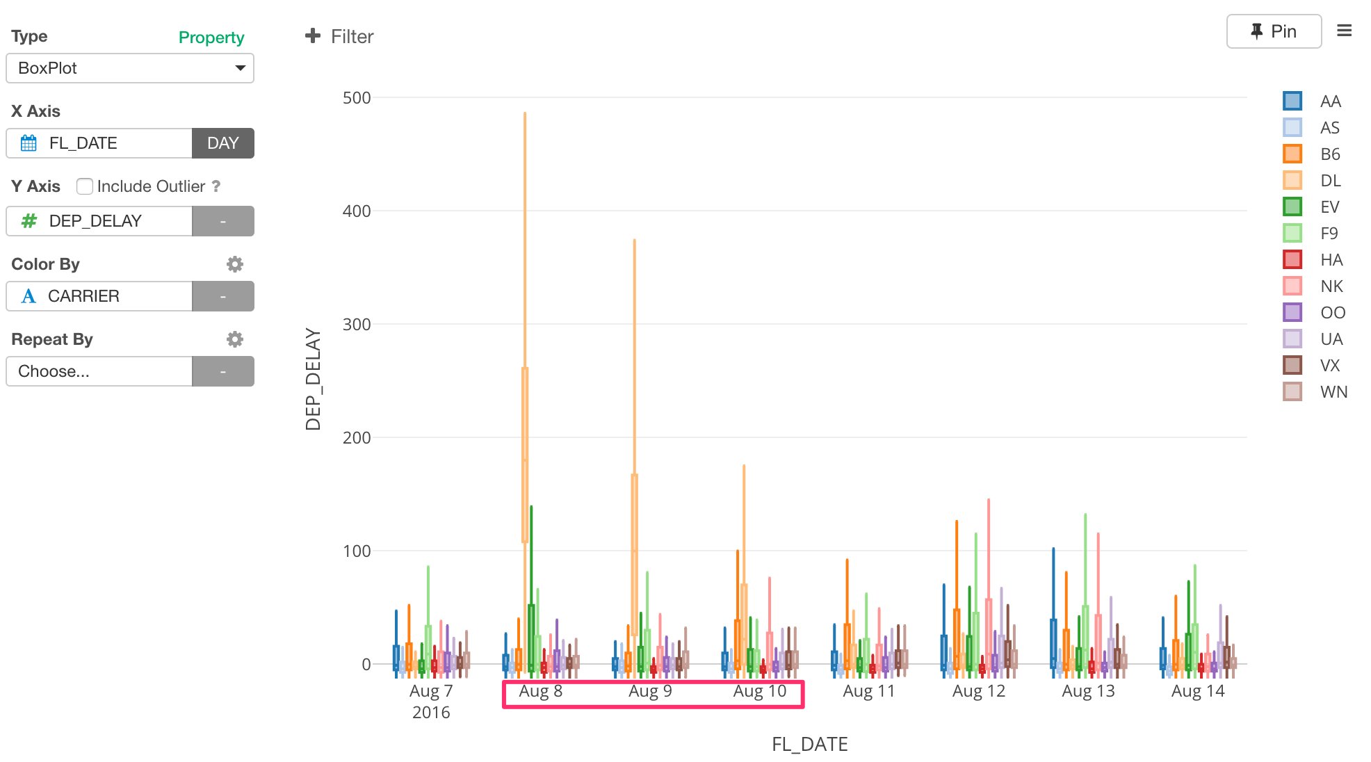
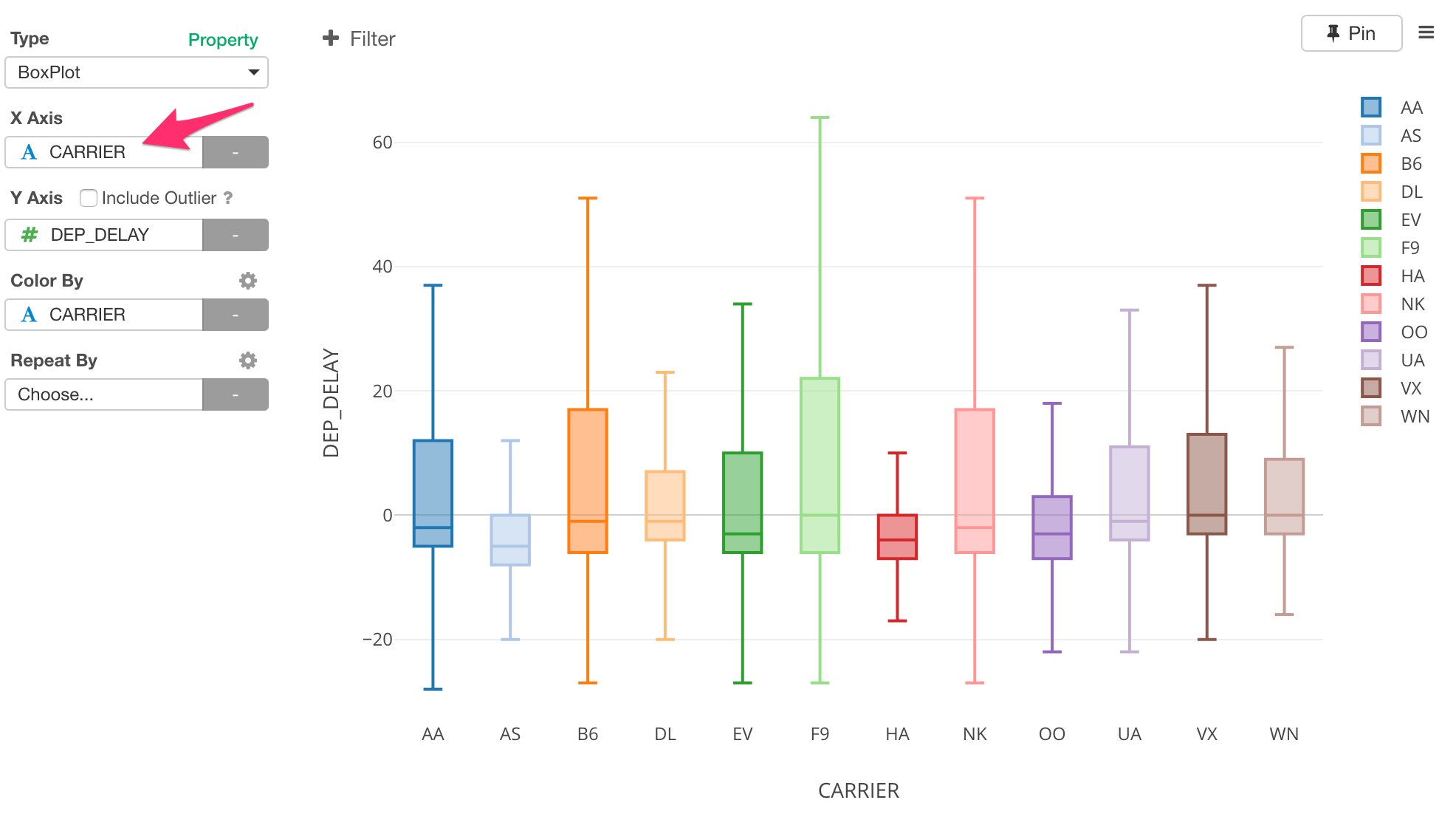
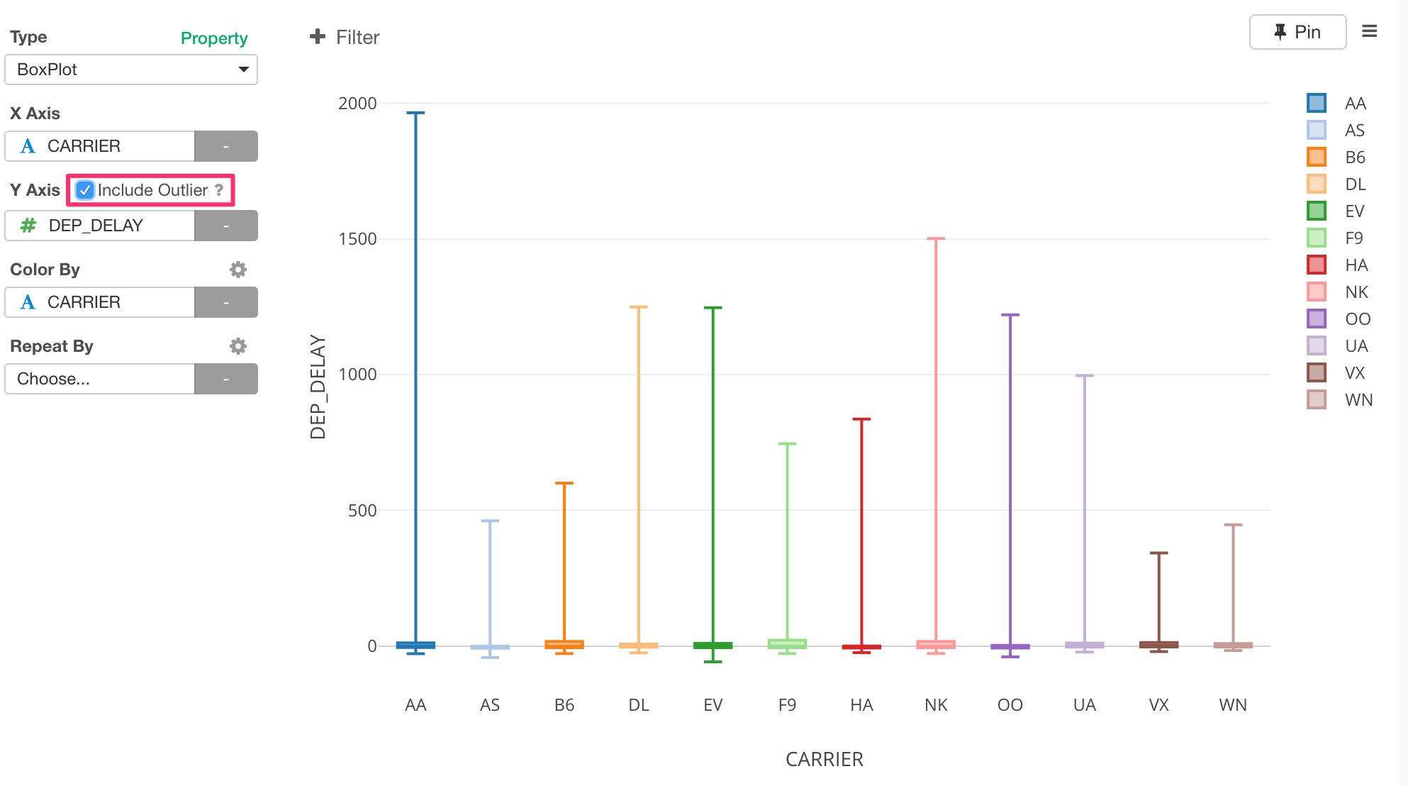
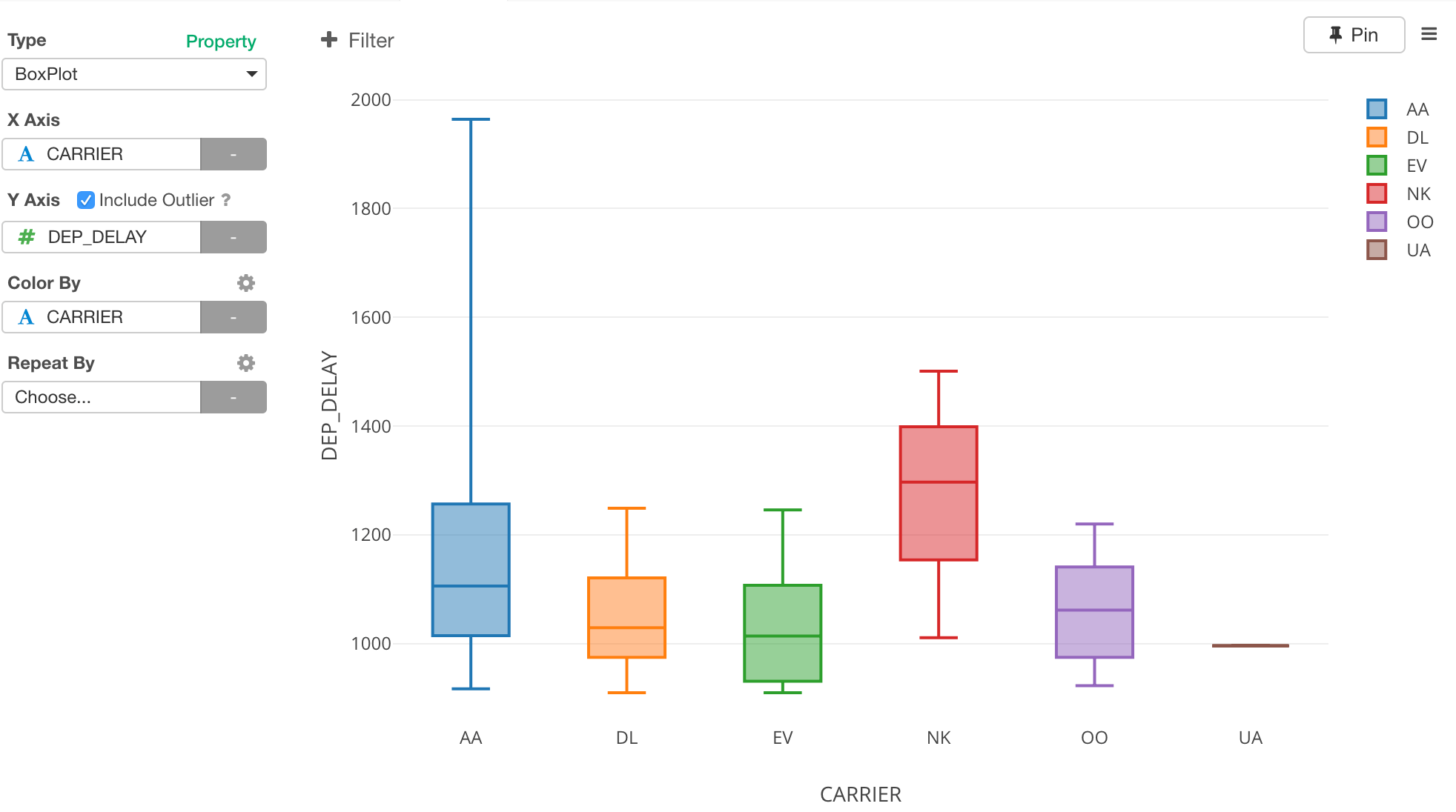
- Boxplot Chart - Understand how bad the flights delayed by each carrier.
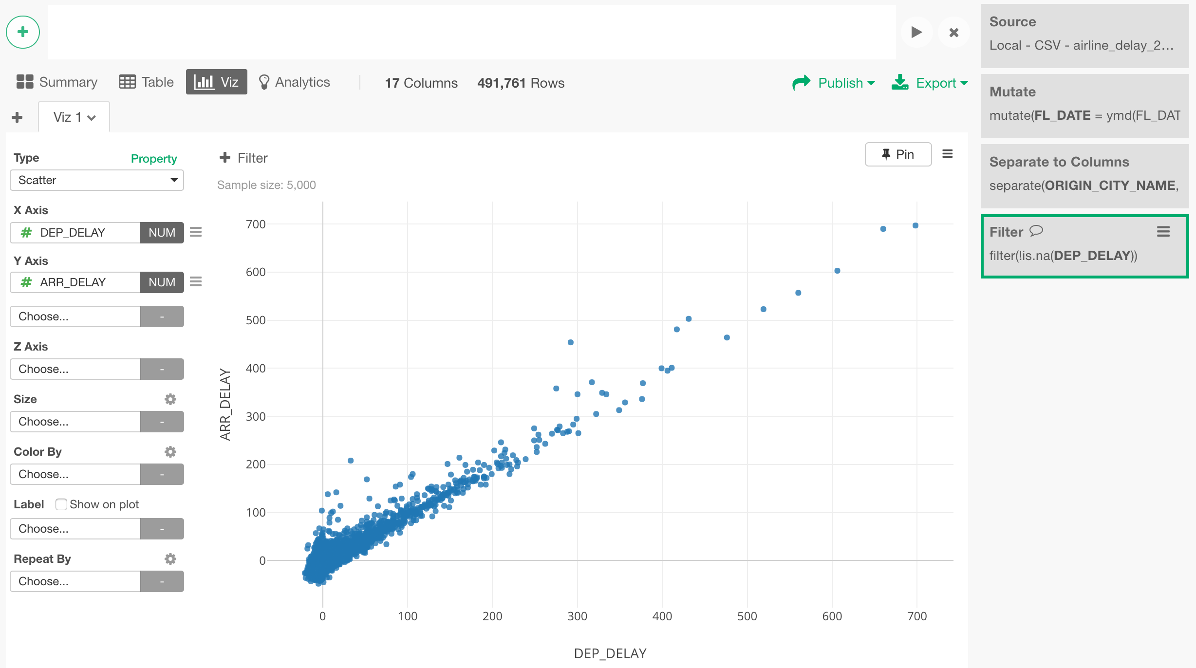
- Scatter Chart - Understand correlations between Arrival Delay and Departure Delay times.
Map with Geocodes (Longitude and Latitude)
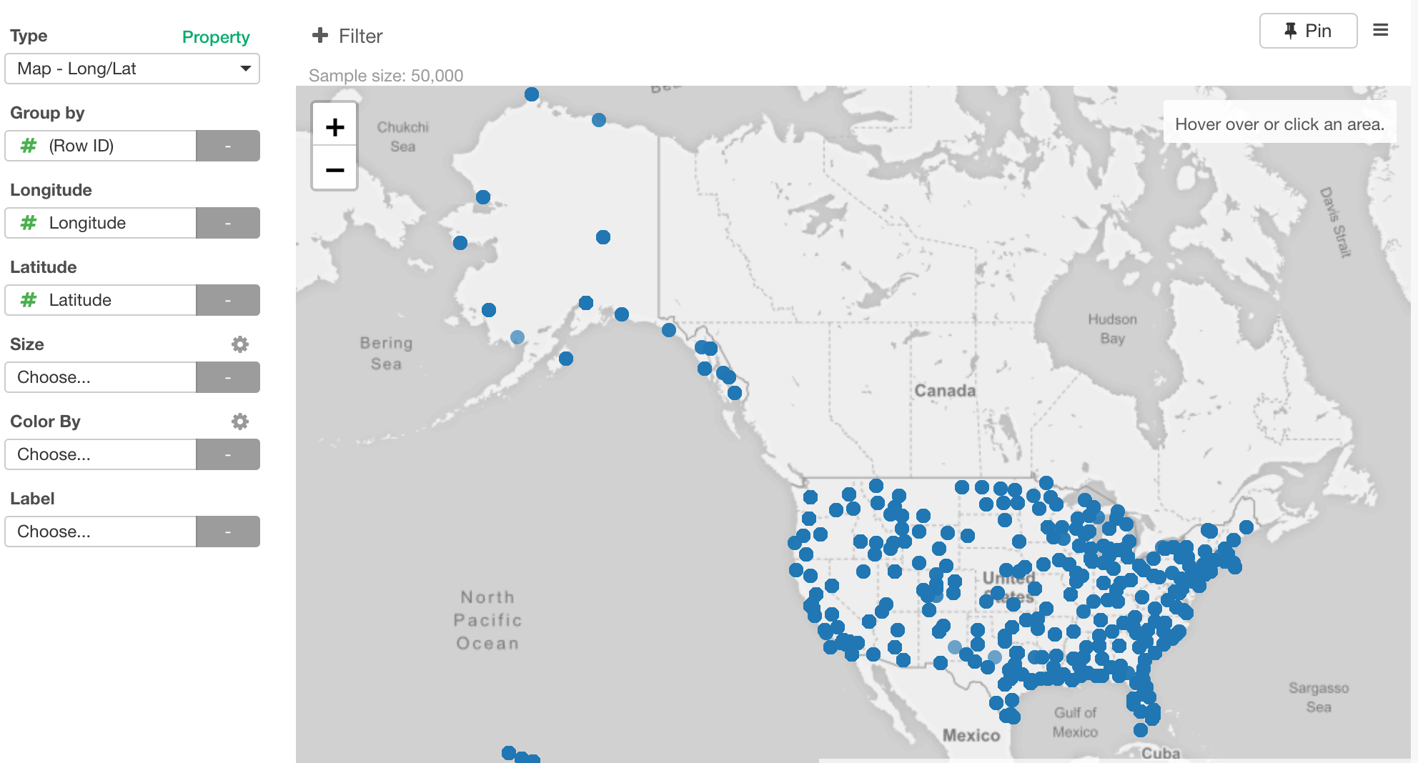
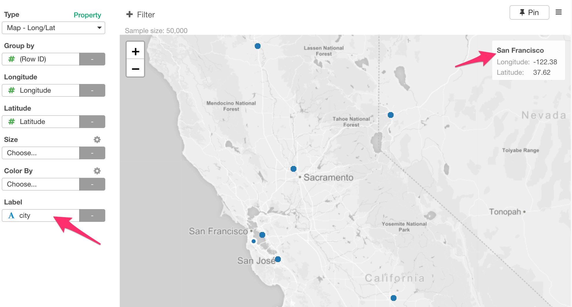
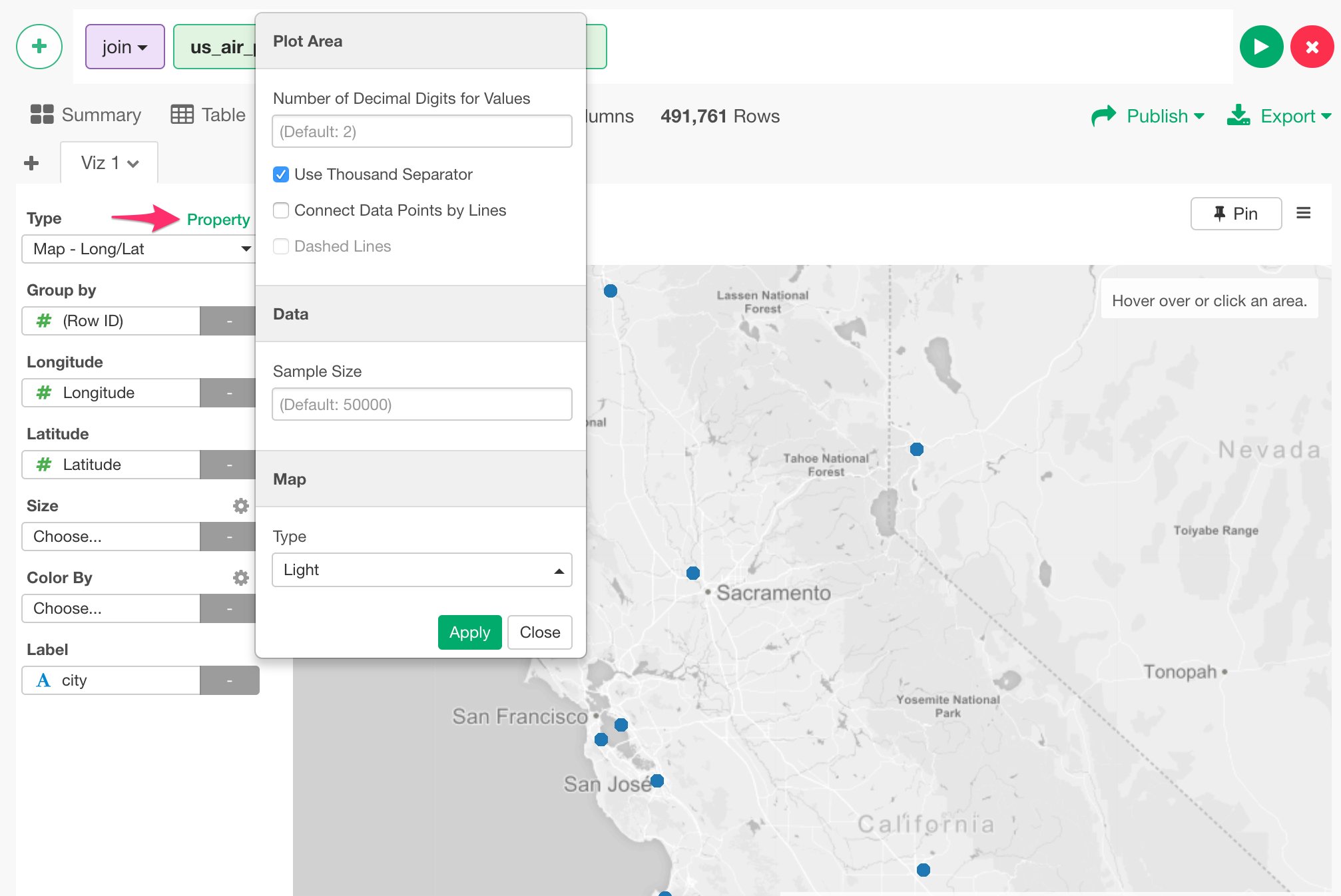
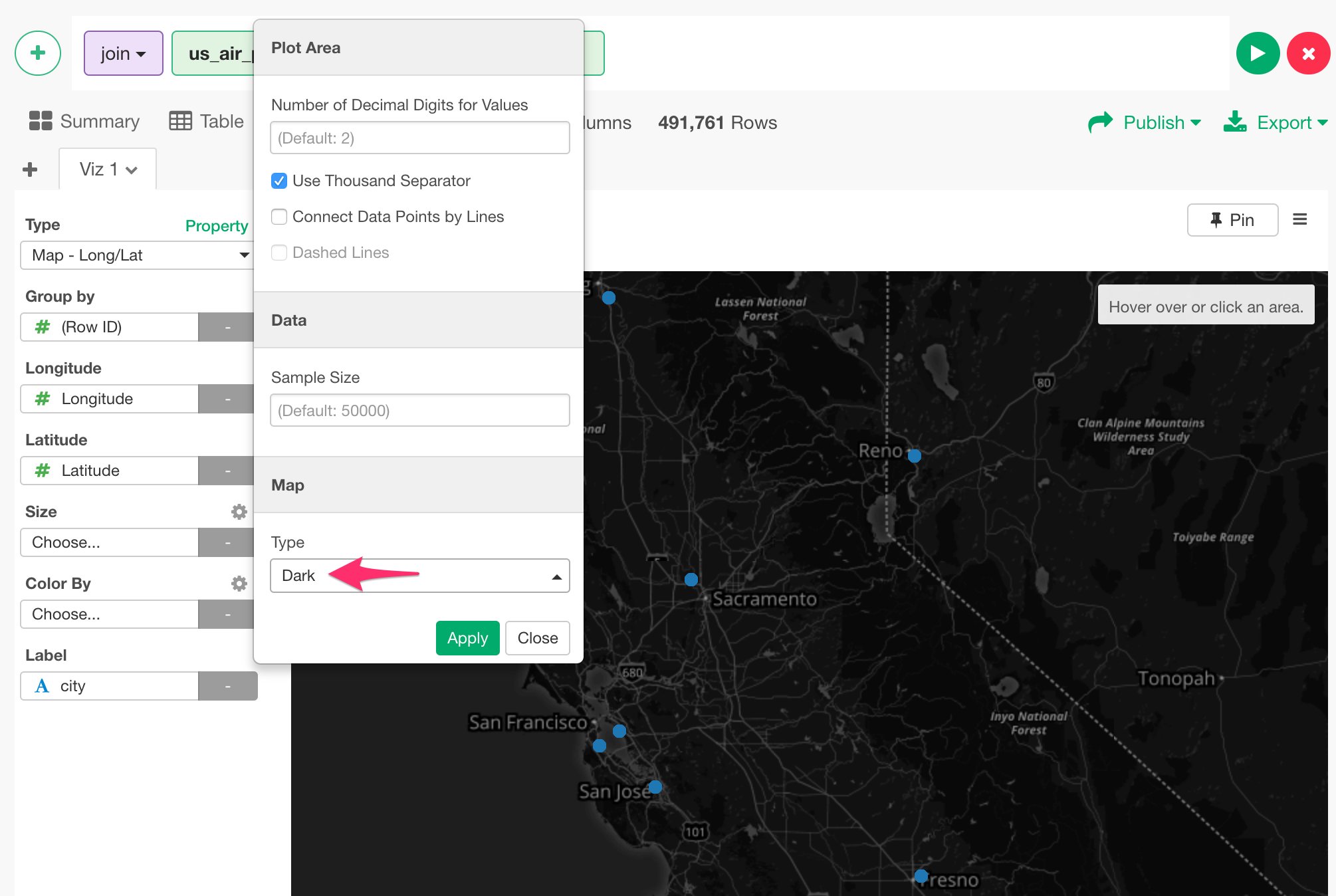
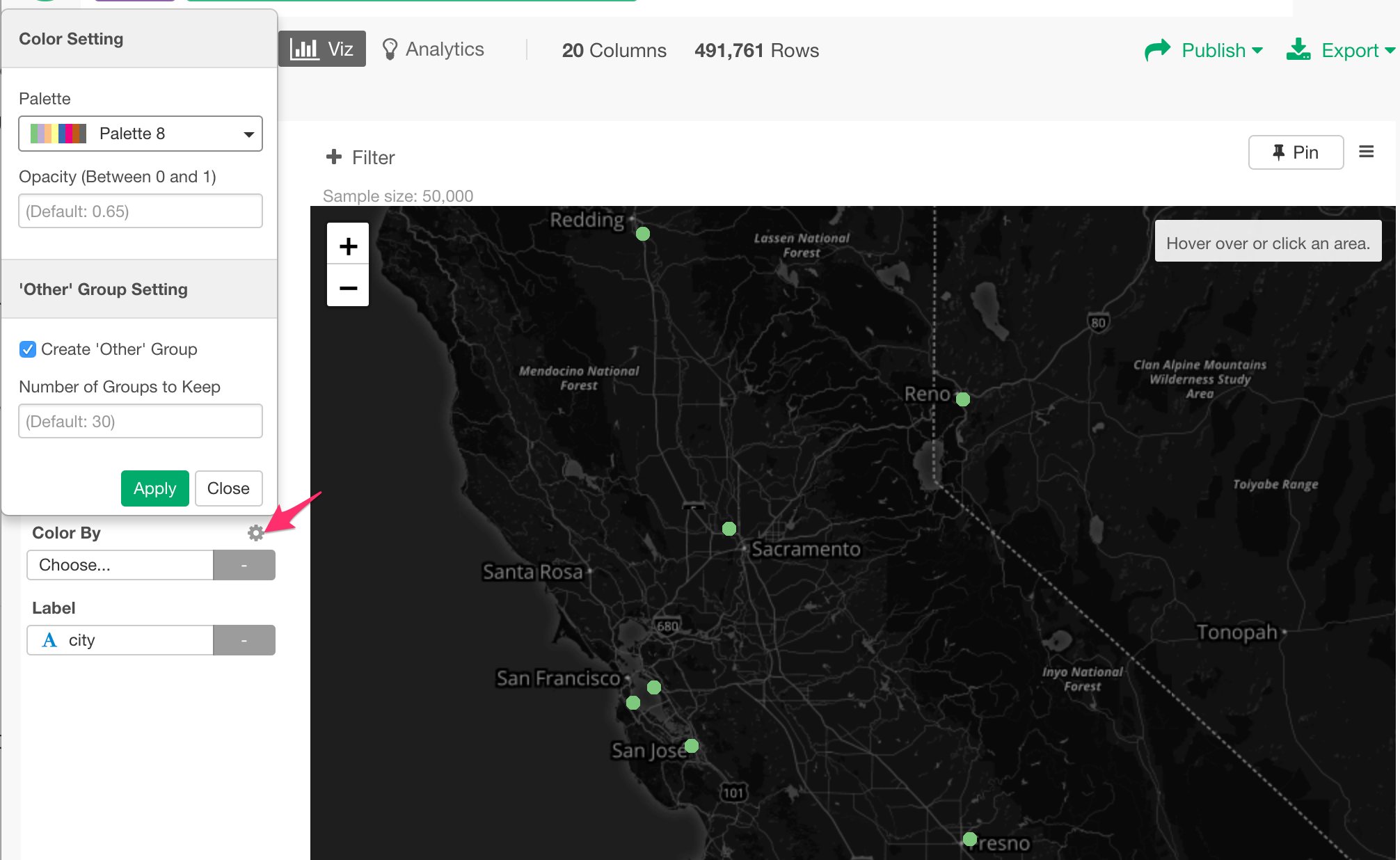
First, let’s take a look at where these flights departed from. Go to Viz view, and select ‘Map - Long / Lat’ chart type.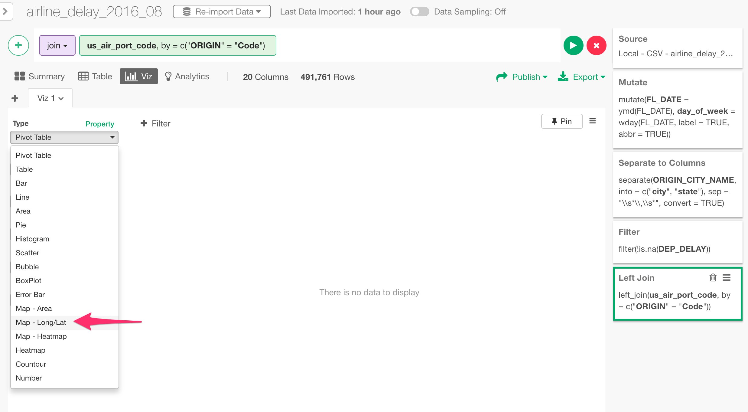
Pivot Table
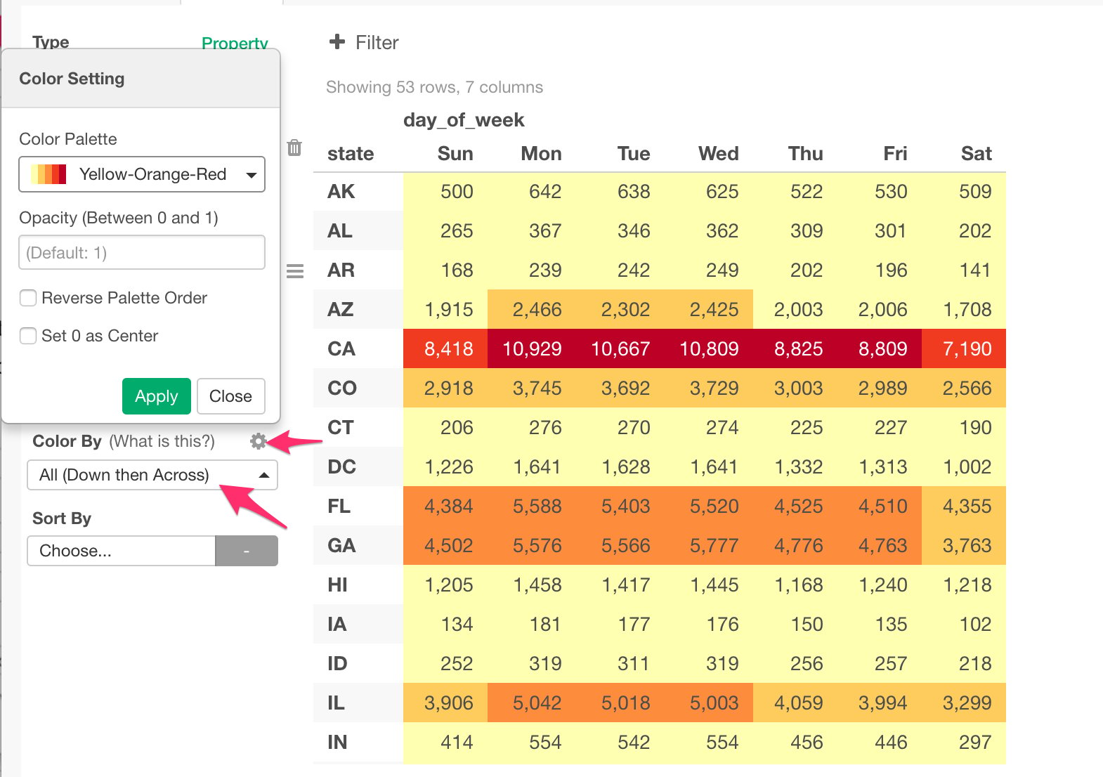
Let’s use Pivot table to understand which state and day pairs have more flights than the others. Select Pivot Table, and assign ‘state’ column to Row and ‘day_of_week’ column to Column. You can keep Value to the default value, which would count ‘Number of Rows’ for each group.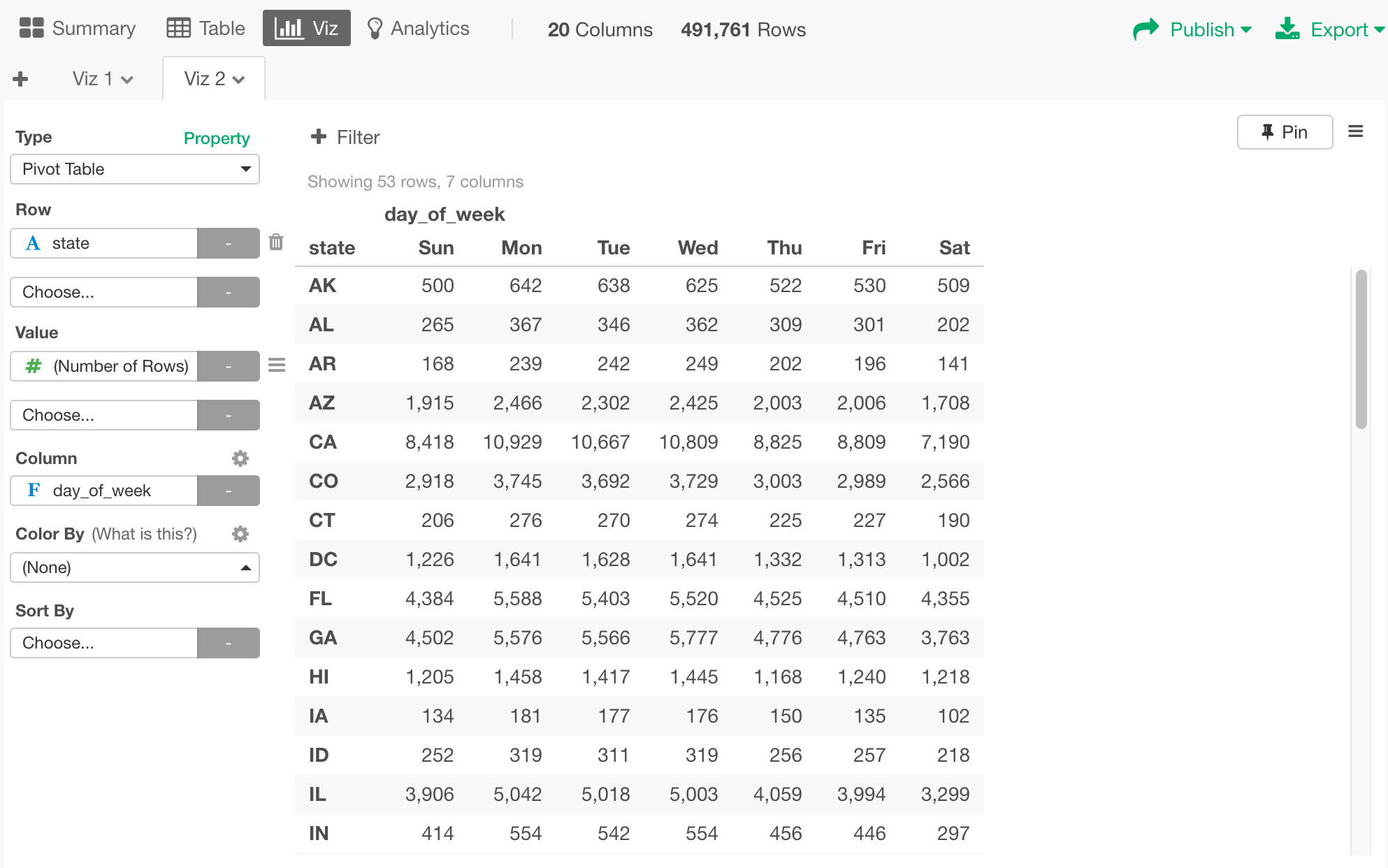
Line Chart / Time Series
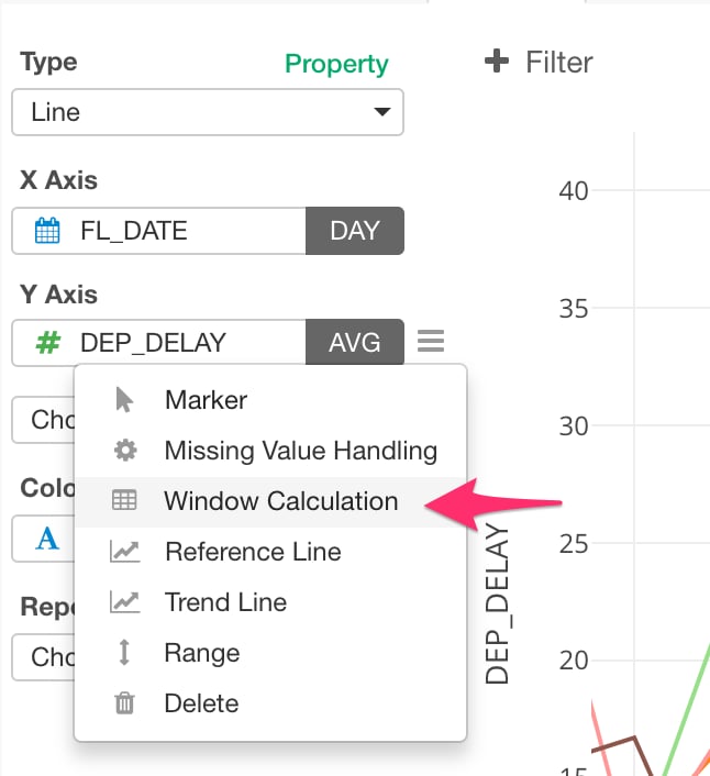
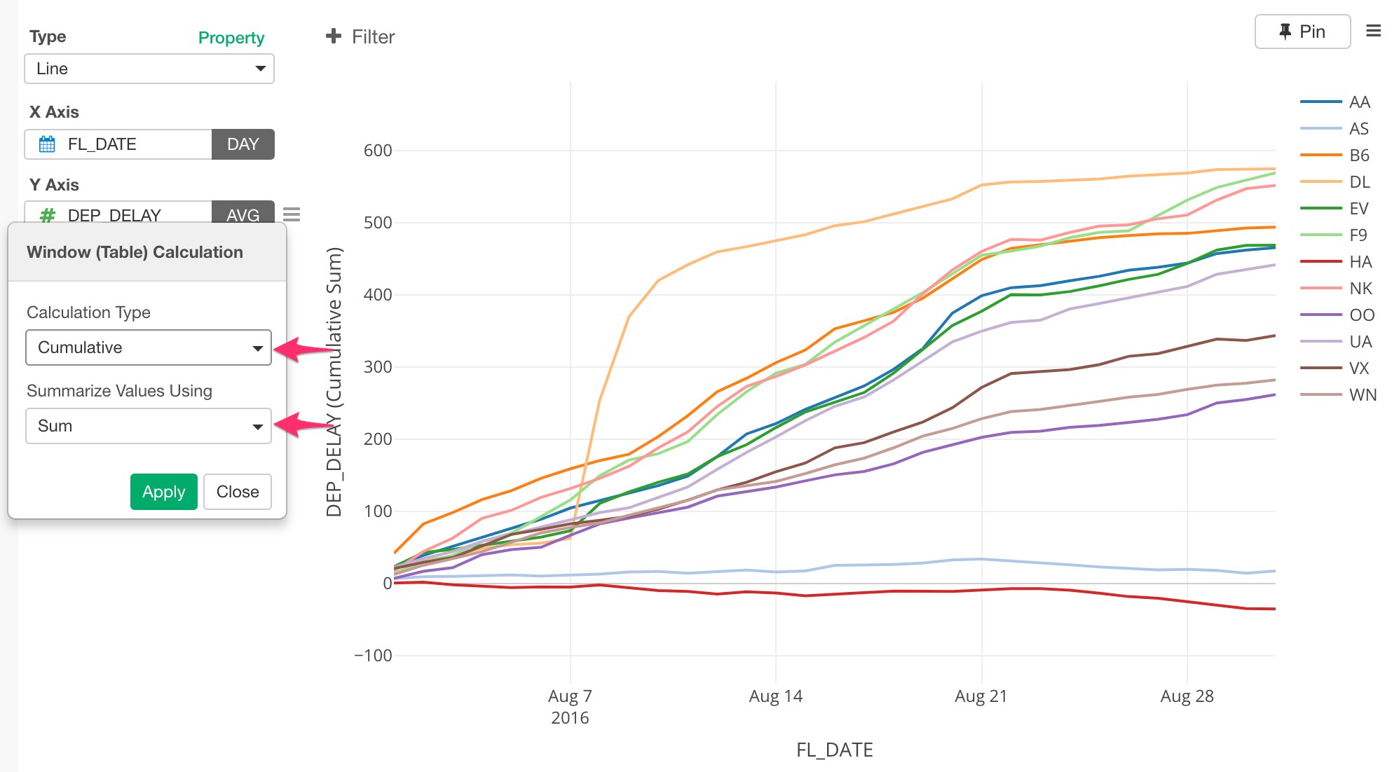
Let’s take a look at the trend of the flight departure delay times during this time period of August, 2016. Select ‘Line’ chart and assign ‘FL_DATE’ column to X-Axis. Since ‘FL_DATE’ column is Date data type, you can select a date level (e.g. Year, Month, Day) to aggregate the data. For example, you can set it to ‘Day’ to aggregate the data by day, instead of the default ‘Year’.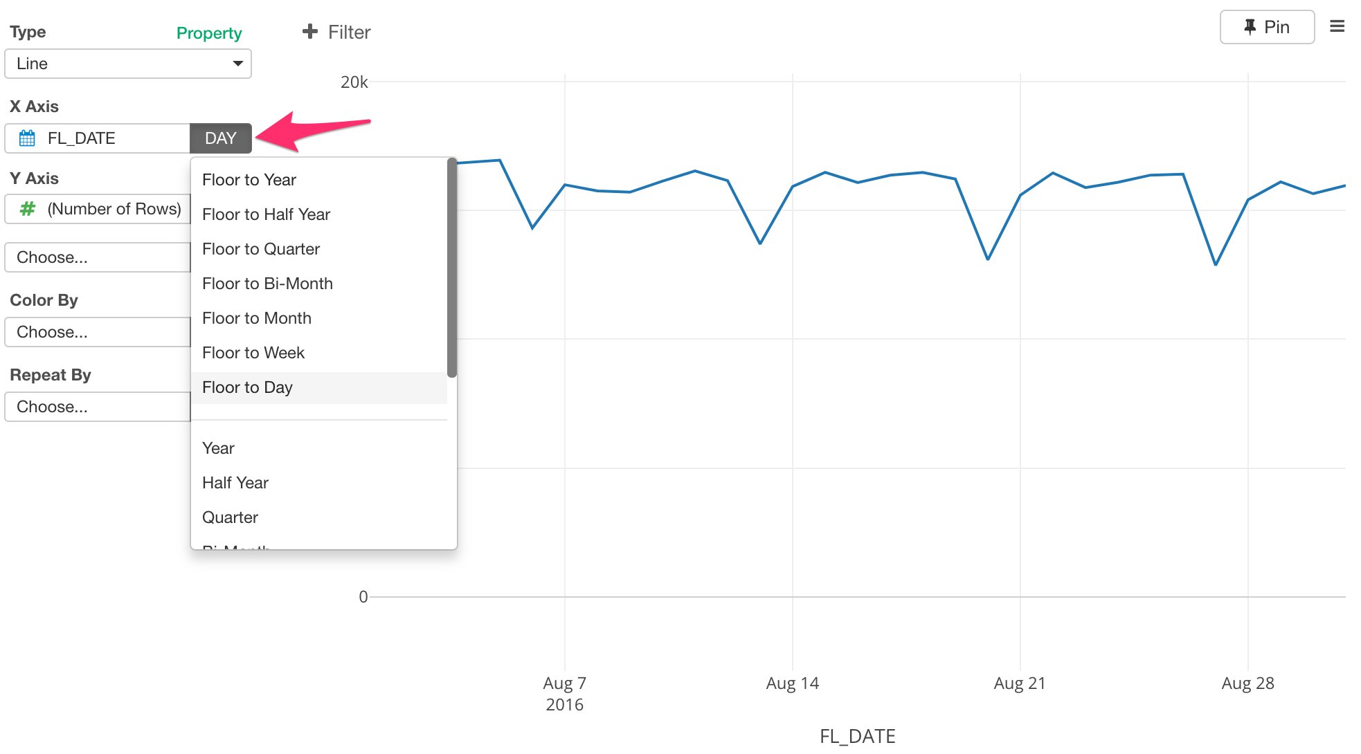
Boxplot
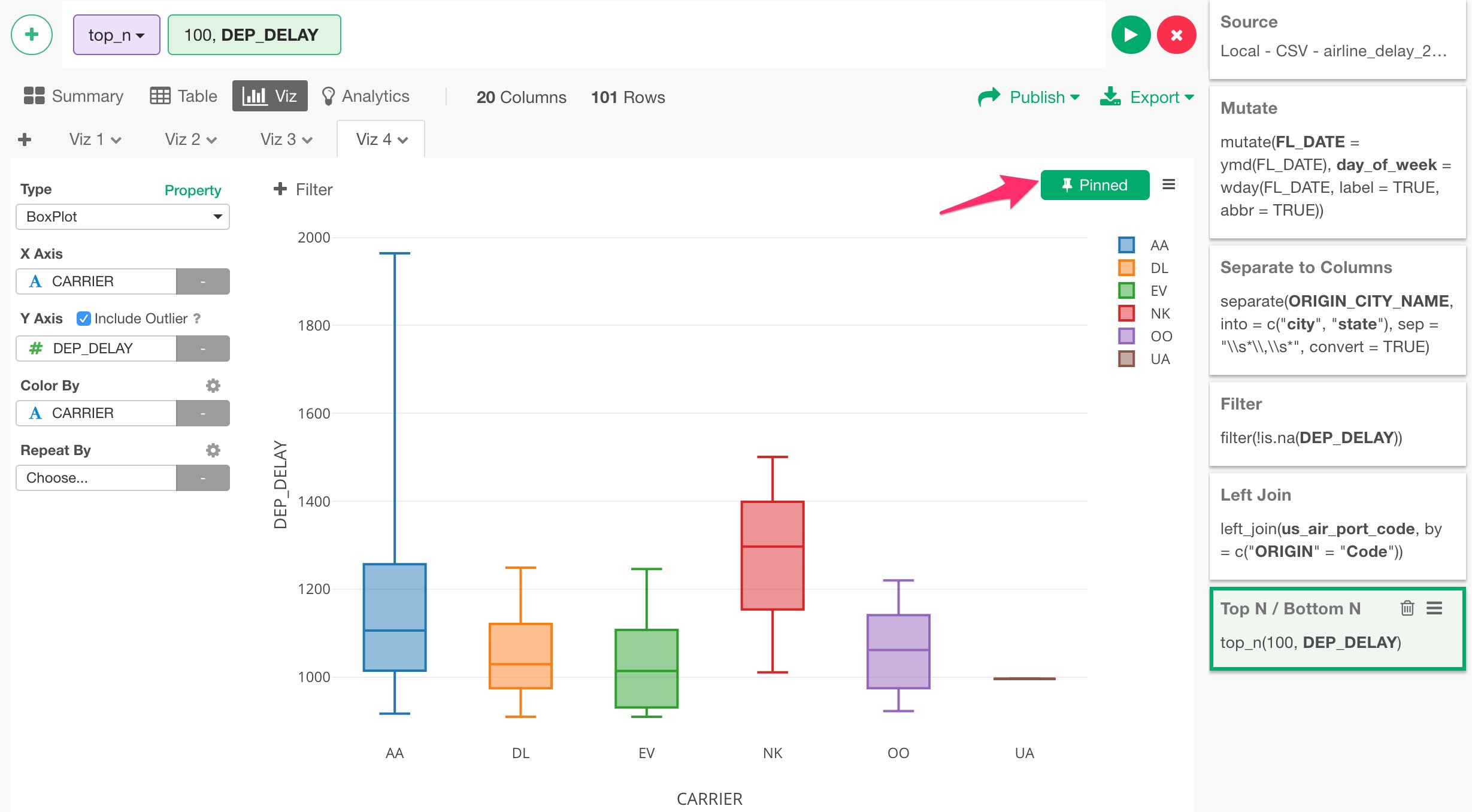
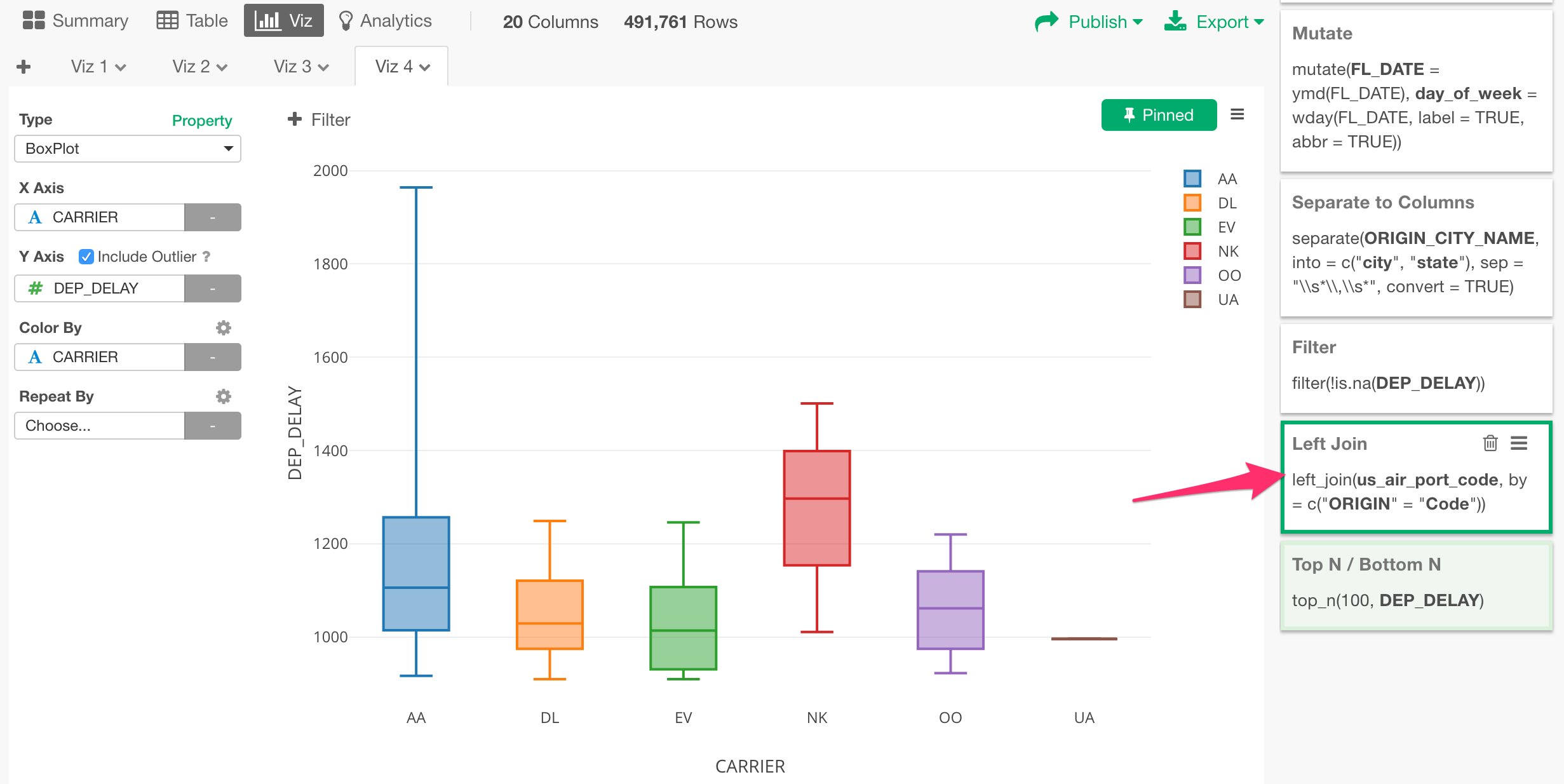
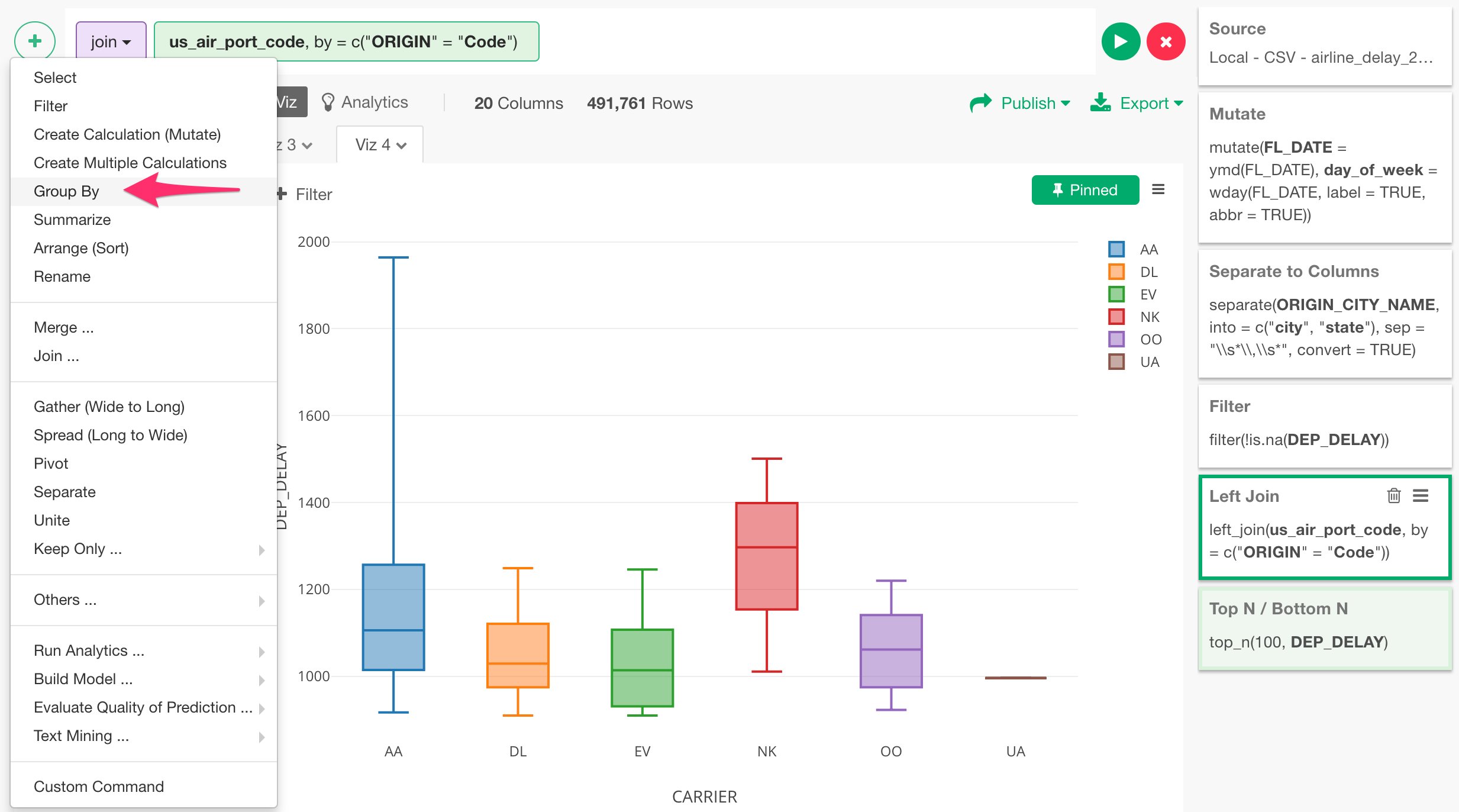
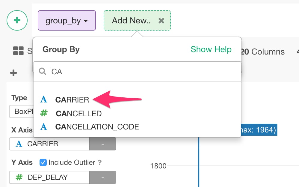
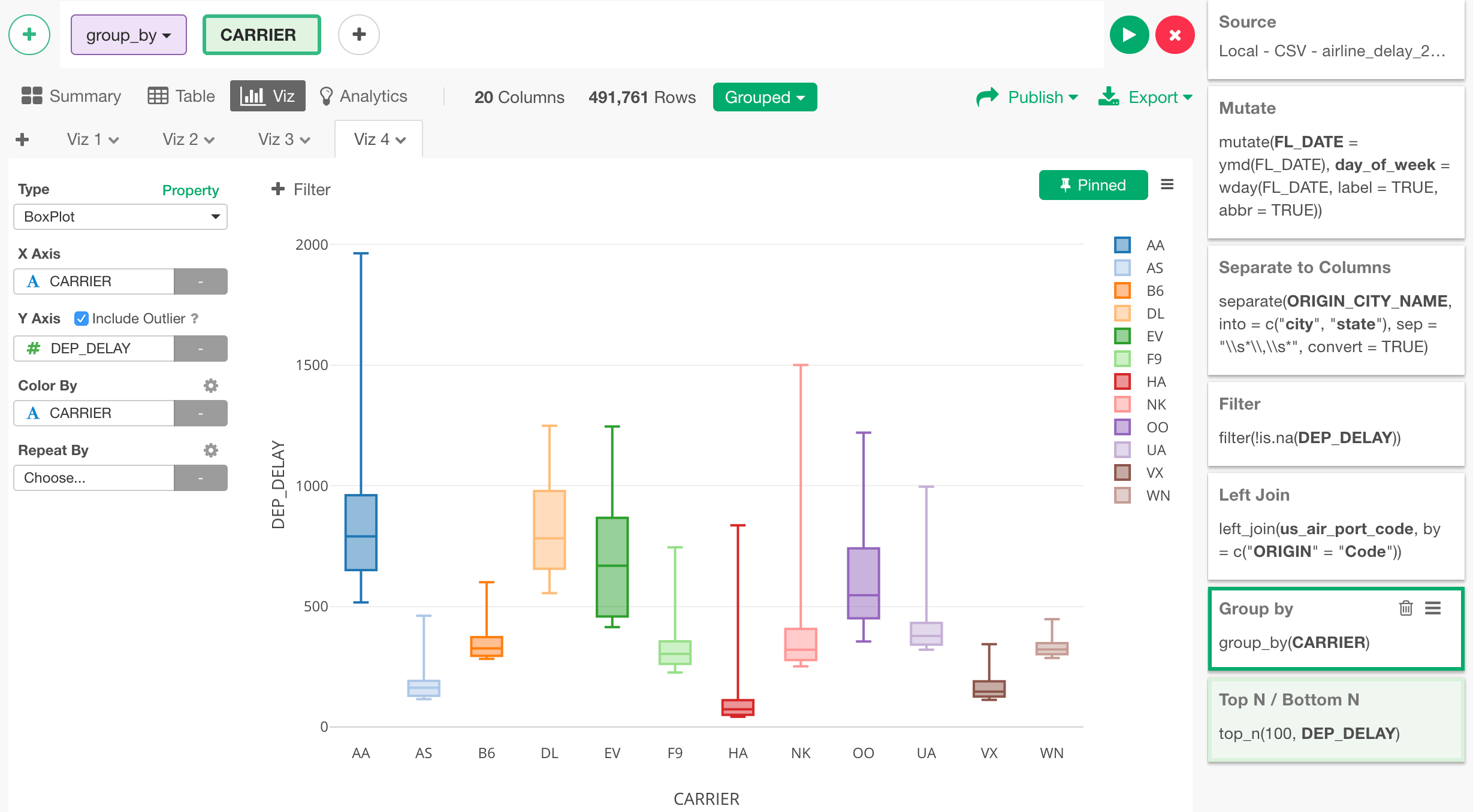
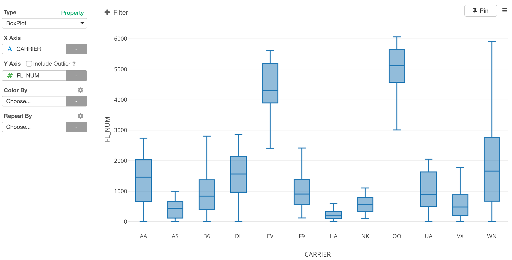
Let’s dig in a little bit more on the departure delay time. We can change the chart type to Boxplot, which would show the data distribution of the departure delay times for each carrier by each day.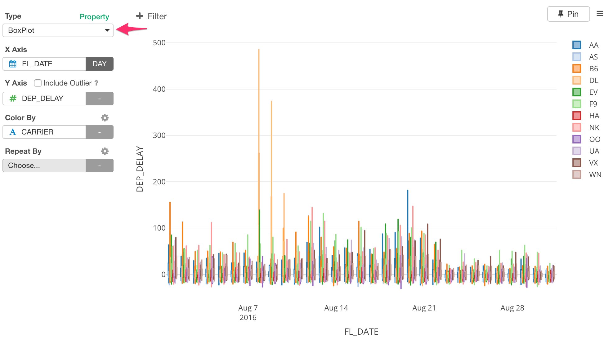
Scatterplot
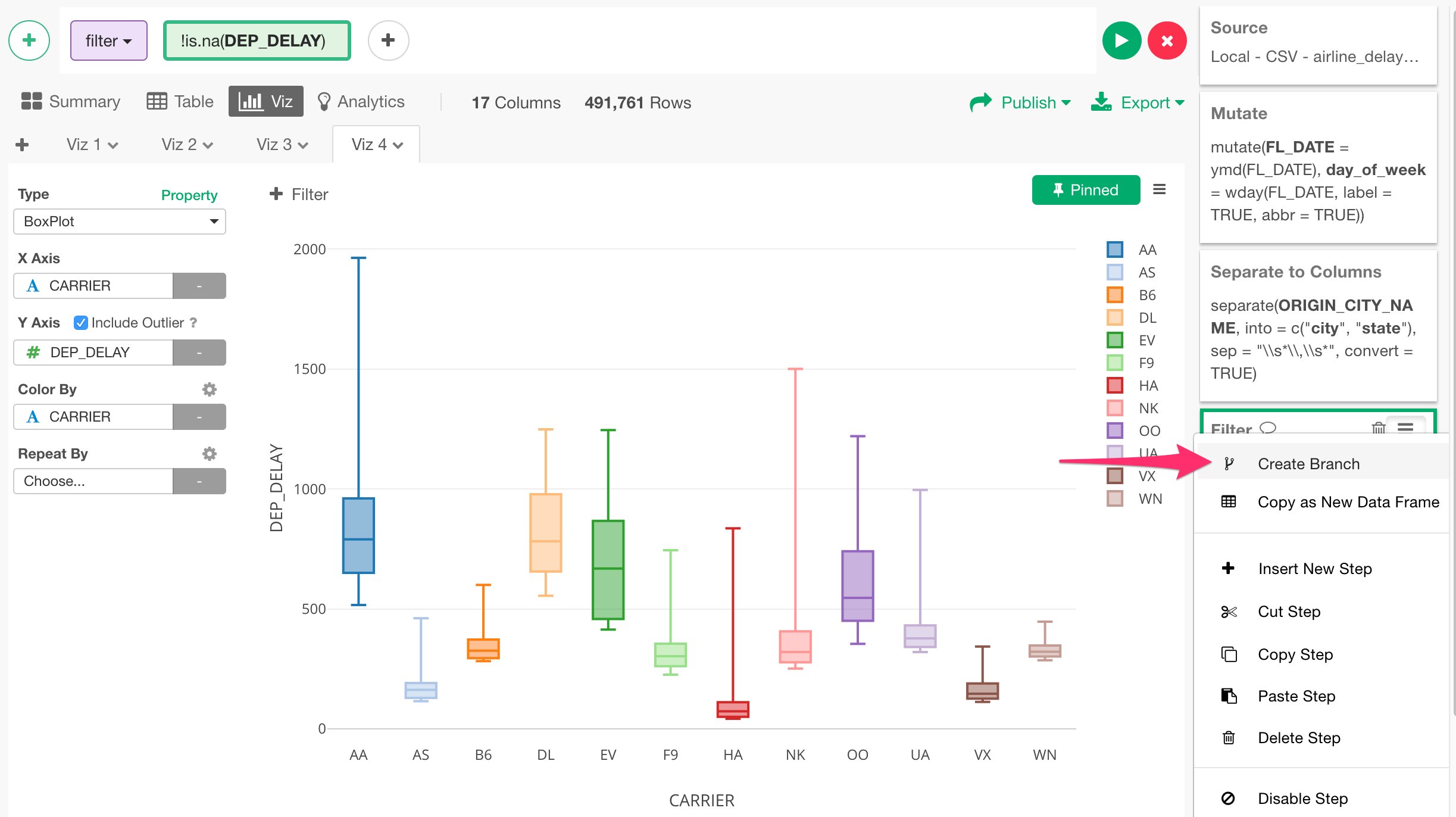
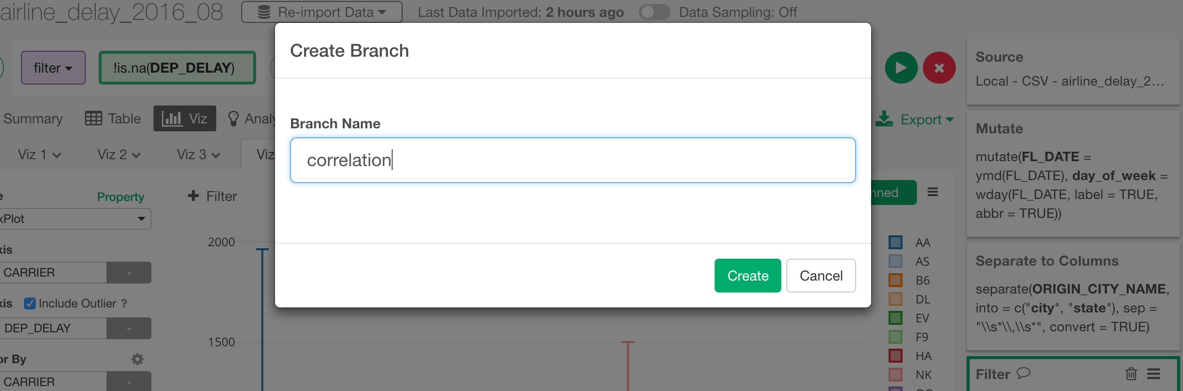
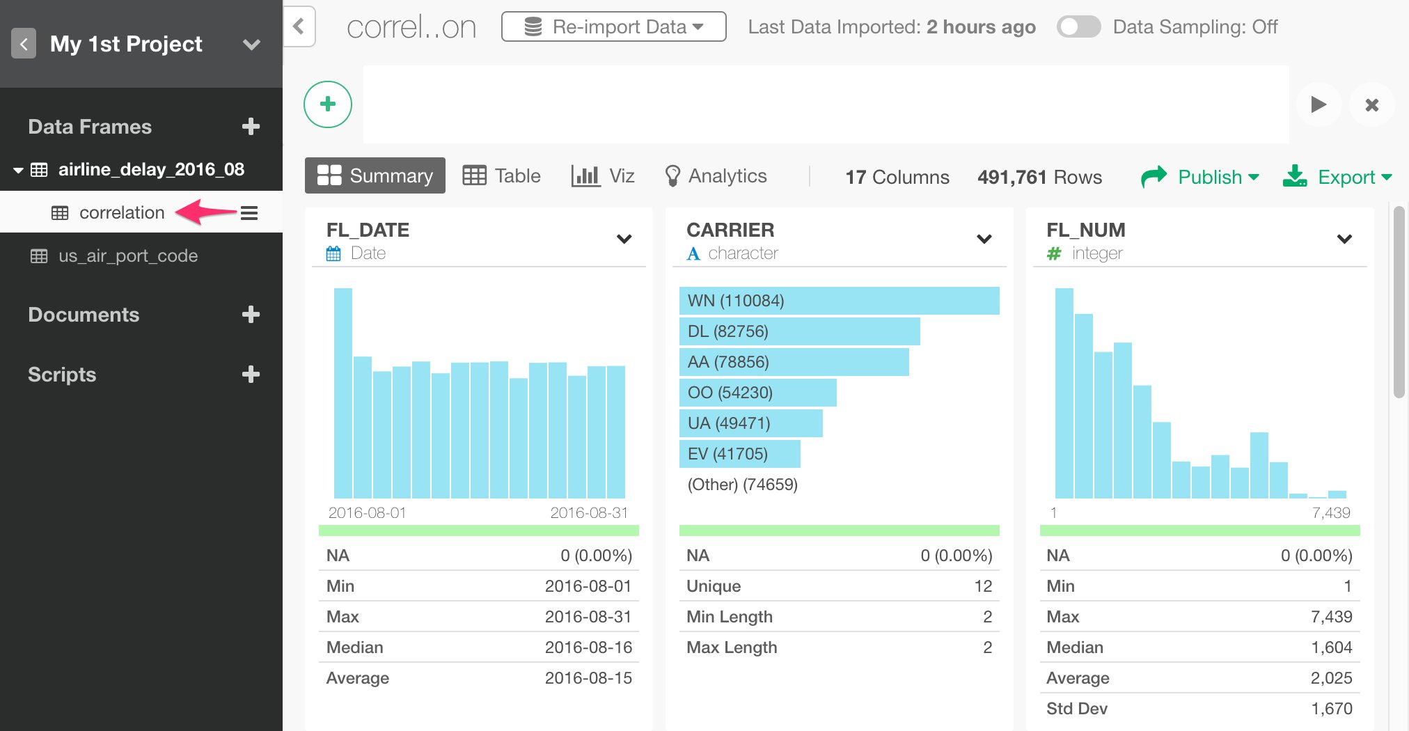
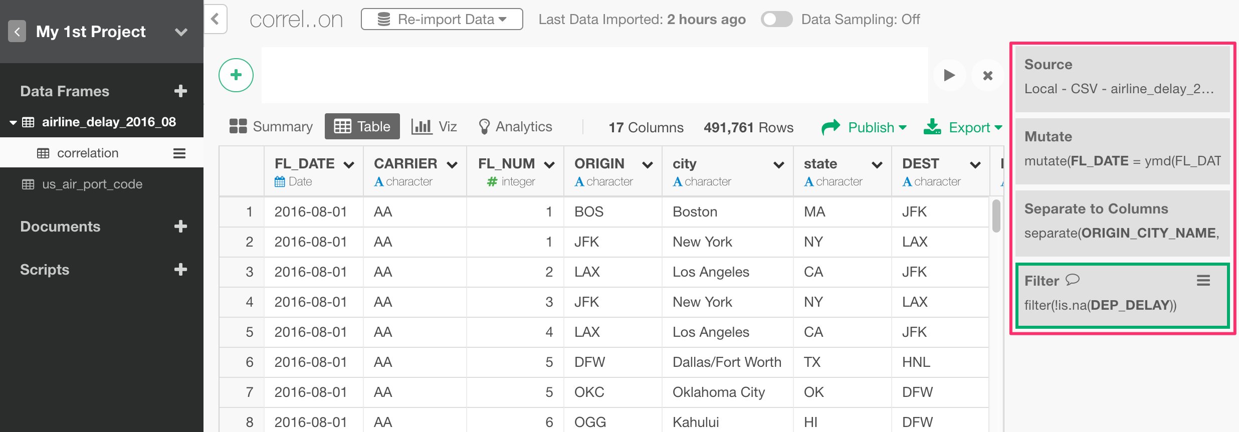
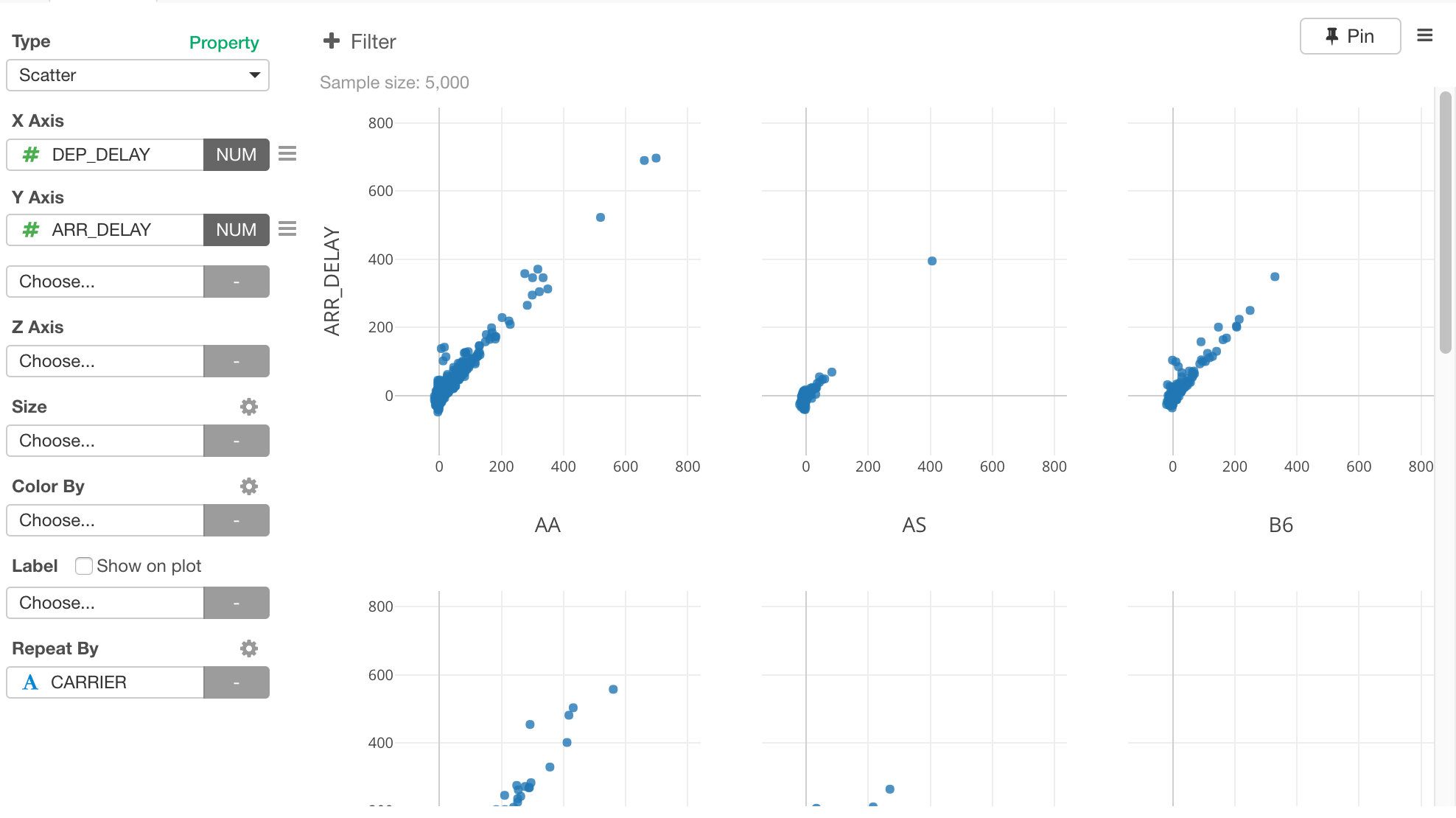
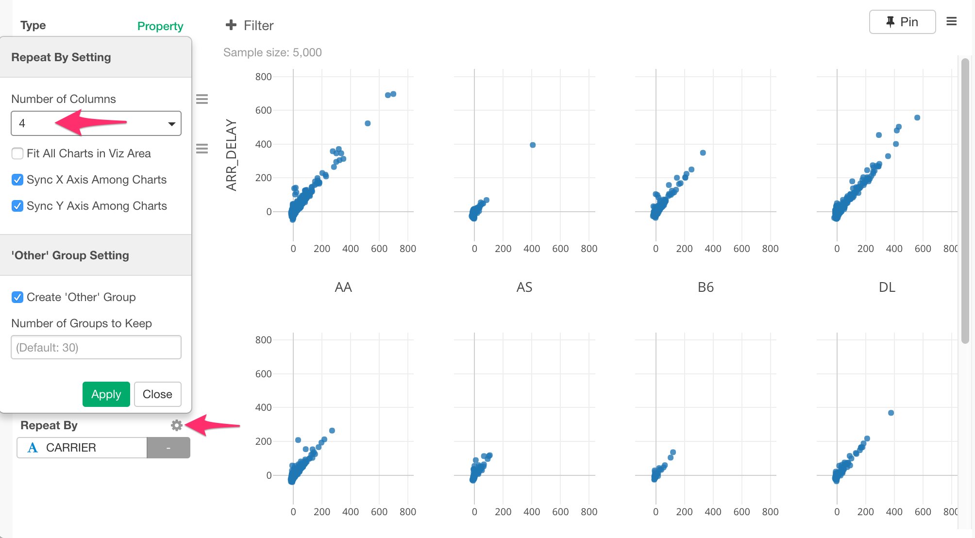
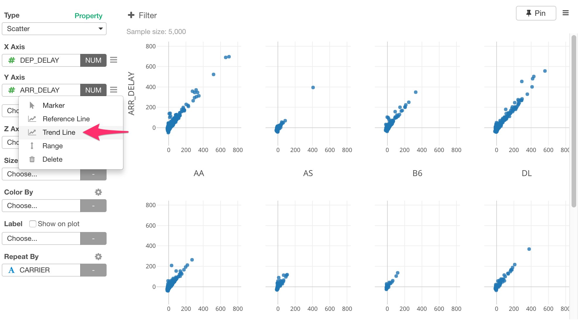
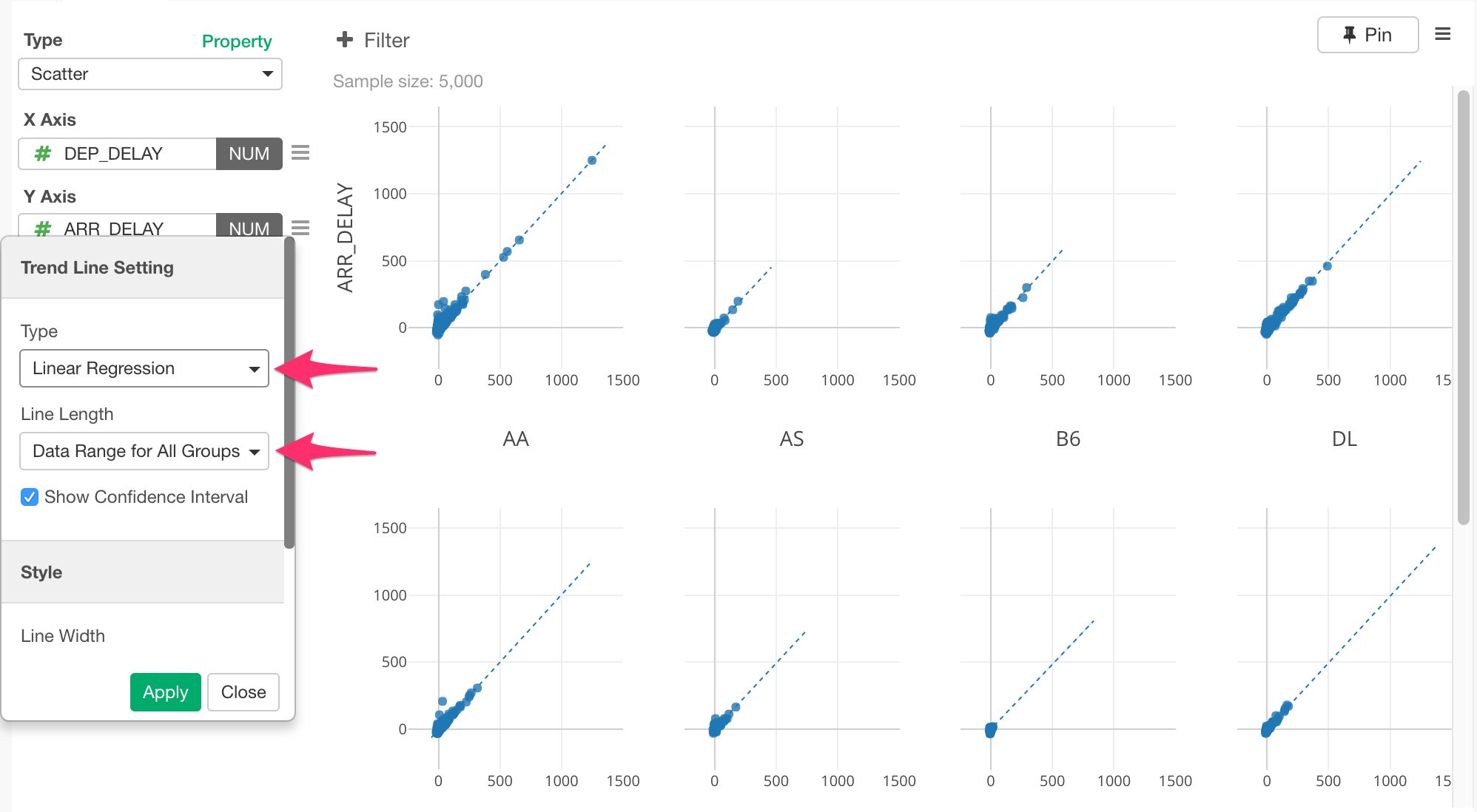
Now, how the departure delay time and the arrival delay time are correlated? In other words, did the flights that delayed for the departure time also delayed for the arrival time? If so, were there any correlation between those two delayed times? To investigate such correlation, we don’t need the last two steps of ‘Group By’ and ‘Top N / Bottom N’ we added previously because we would rather evaluate the entire data. So for this analysis, instead of deleting these two steps, we can create something called ‘branch’ data frame off from the step before ‘Group By’ step. This way, we can create two data frames with two different data wrangling paths while sharing the common part of the data wrangling steps. Select ‘Filter’ step at the right hand side.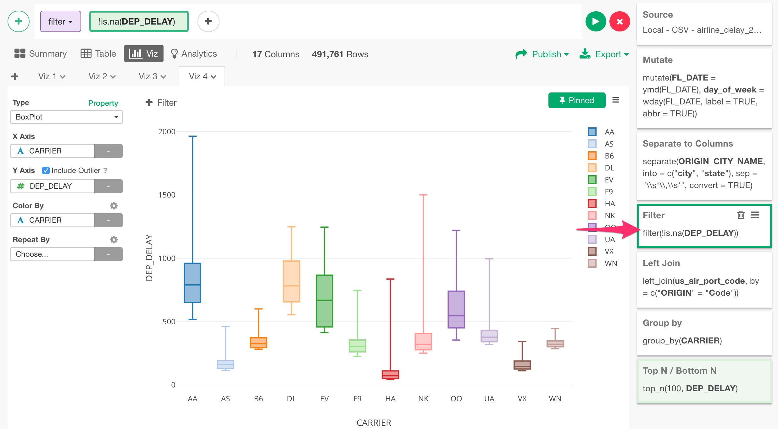
Use Machine Learning Algorithm to Gain Deep Insights
Variable Importance with Random Forest
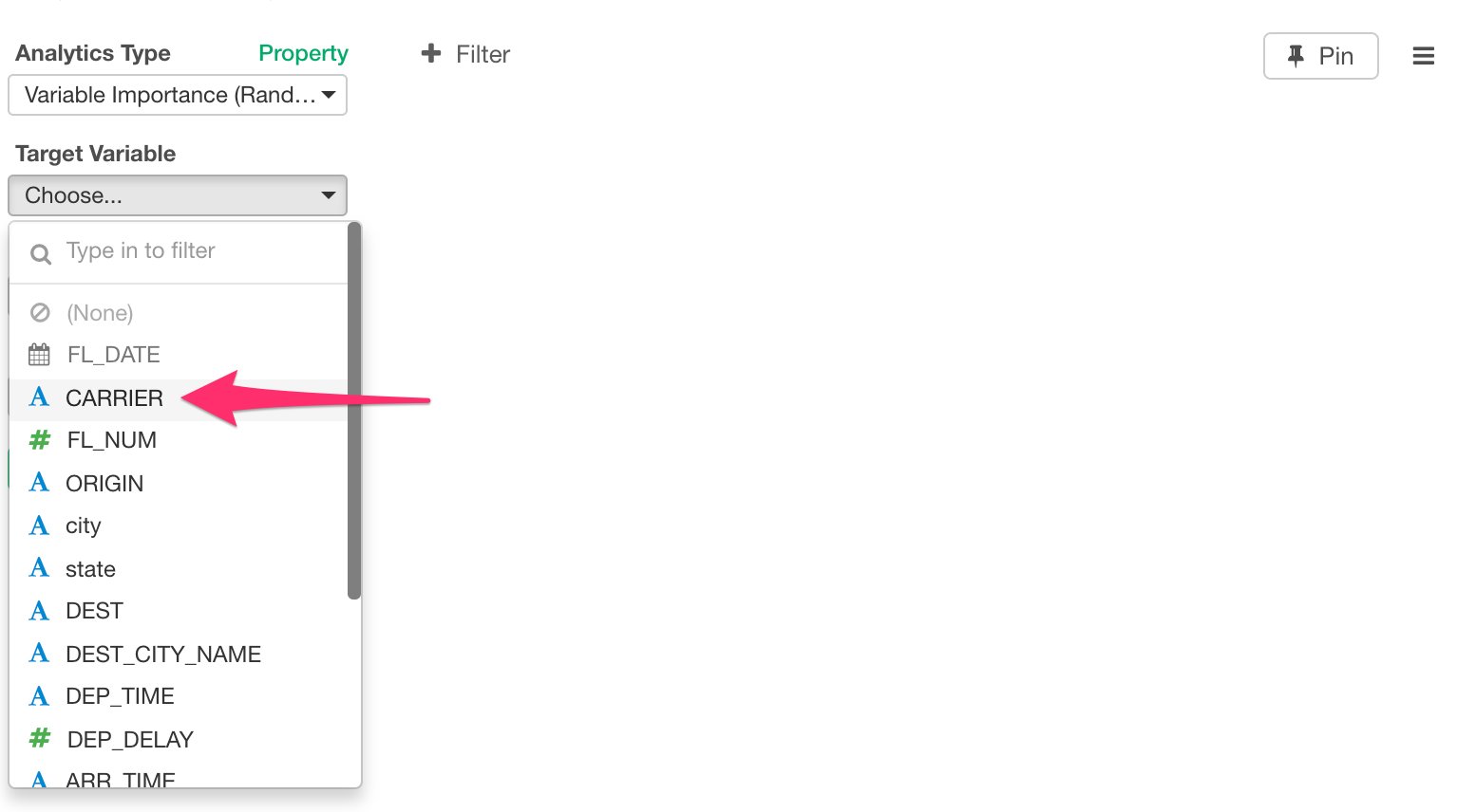
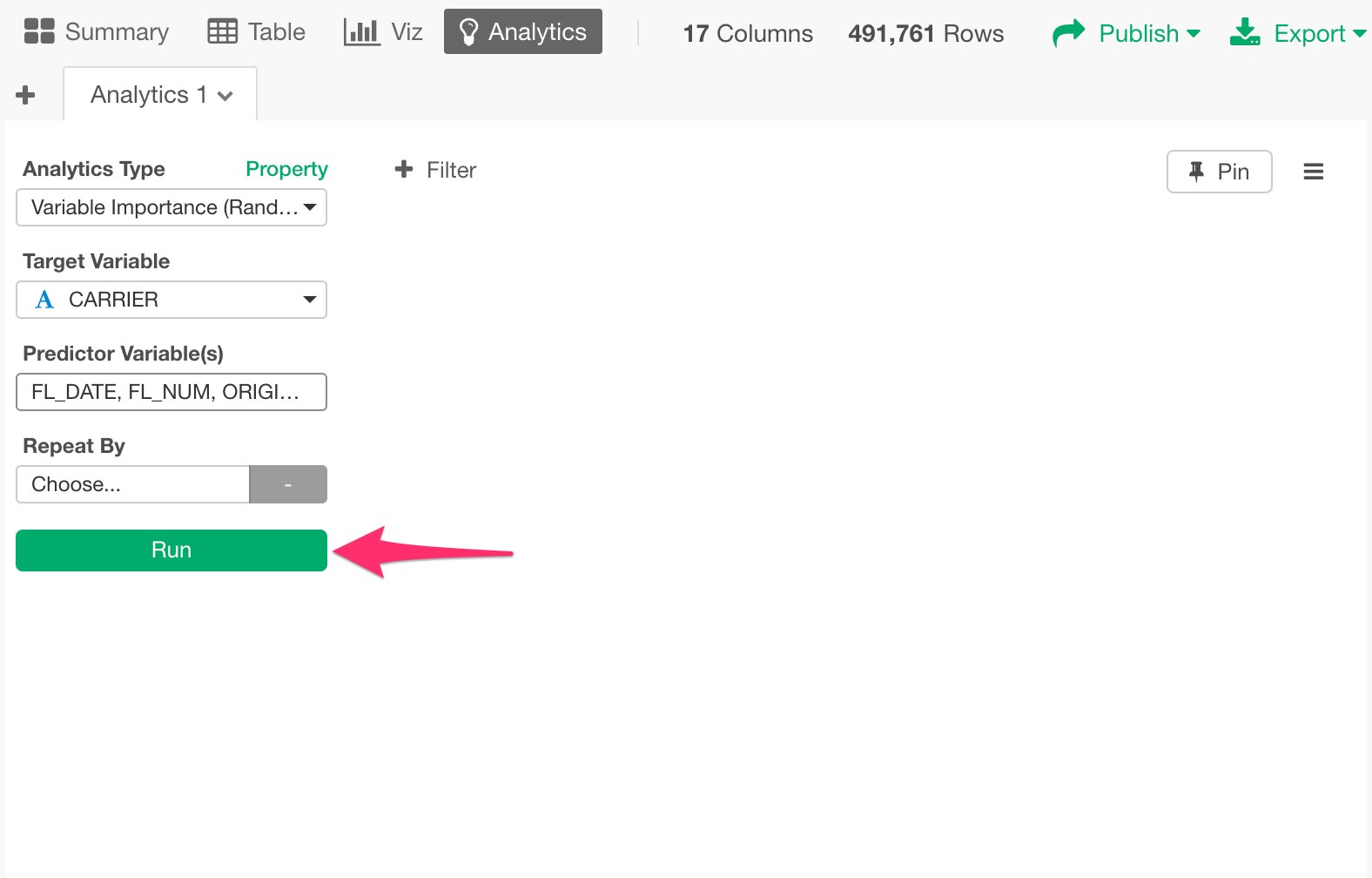
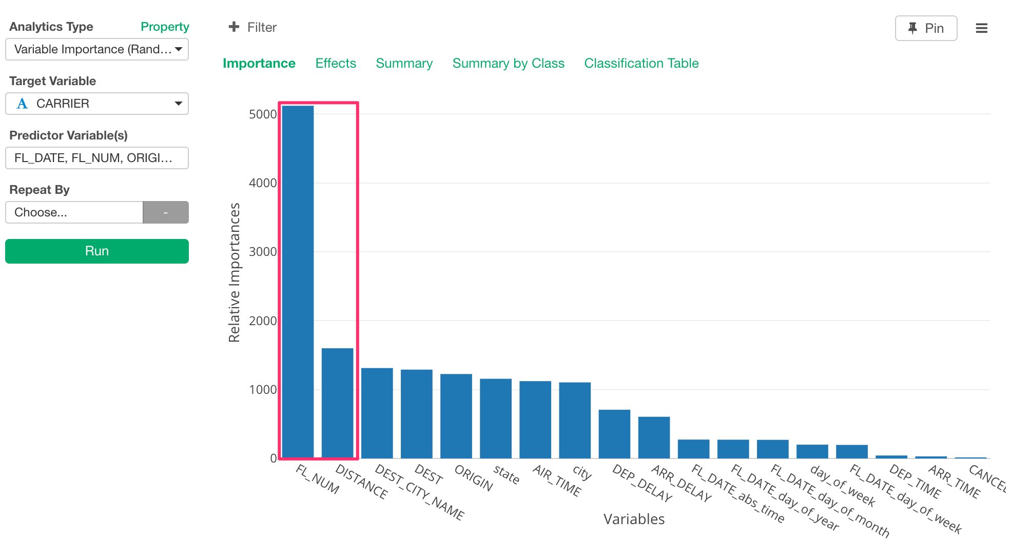
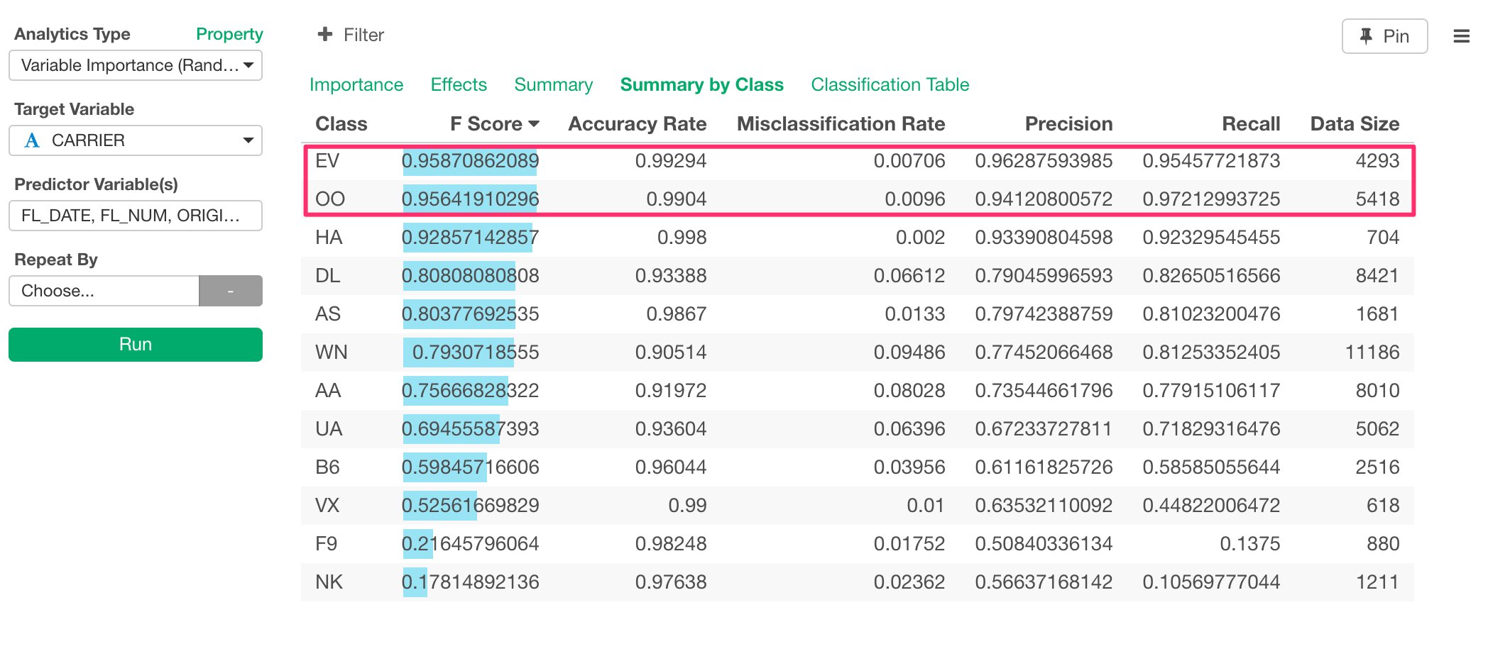
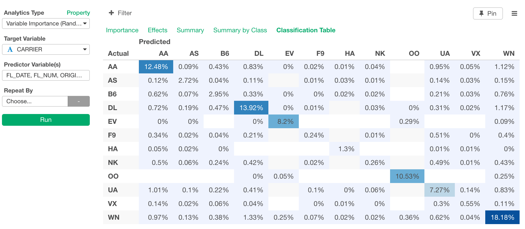
Visualization is great when you can recognize the patterns and trends with your eyes. But most often than not, things are not that simple. For example, out of all these columns (or variables) like FL_DATE, ARR_DELAY, DEP_DELAY, FL_MUM, DISTANCE, etc, which are the most useful to characterize the carrier? In other words, if we don’t have CARRIER column, can we still predict which carrier is for any given row of the flight data? You can answer to this type of questions by using Machine Learning or Statistical algorithms. In Exploratory, you can use ‘Variable Importance’ feature under Analytics view. This internally uses Random Forest algorithm and help you find which columns are more influential in terms of predicting the outcome that you are interested. First, click Analytics Tab and select ‘Variable Importance’ from Analytics Type pulldown list.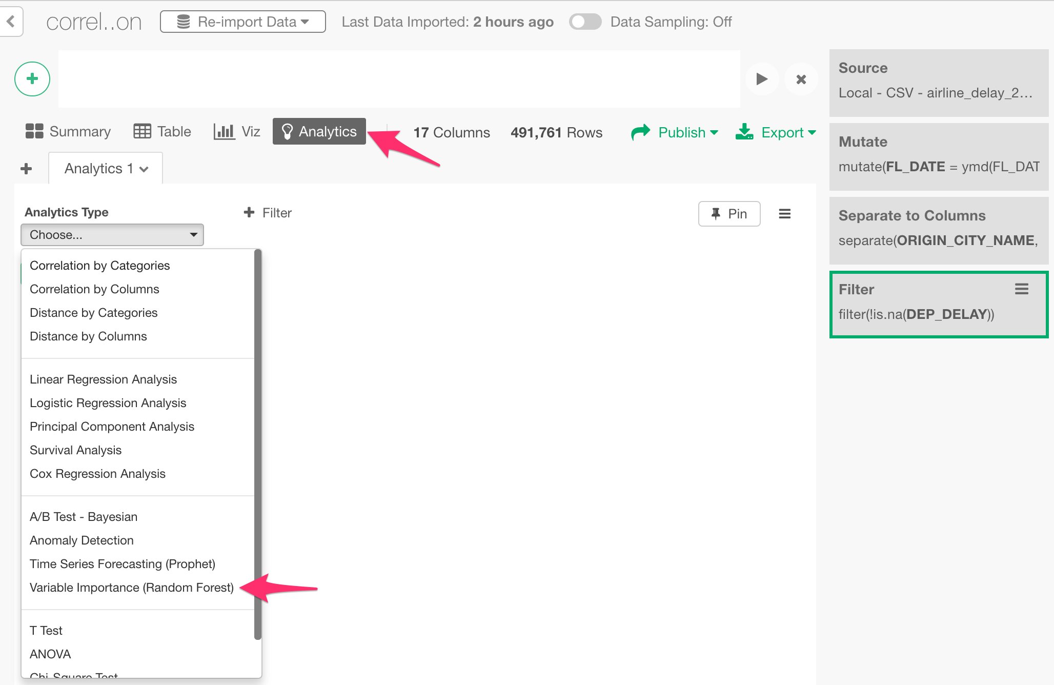
Share Chart
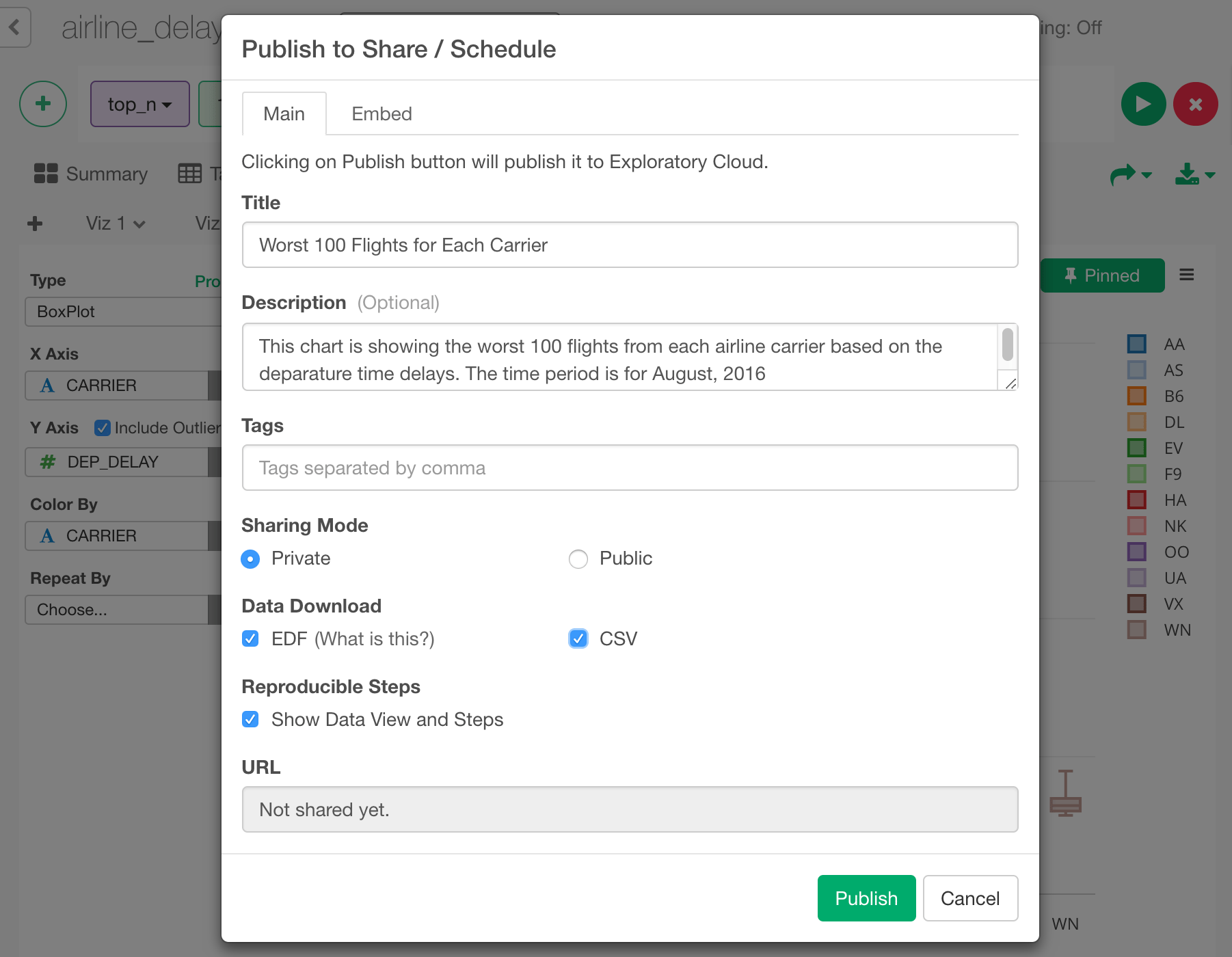
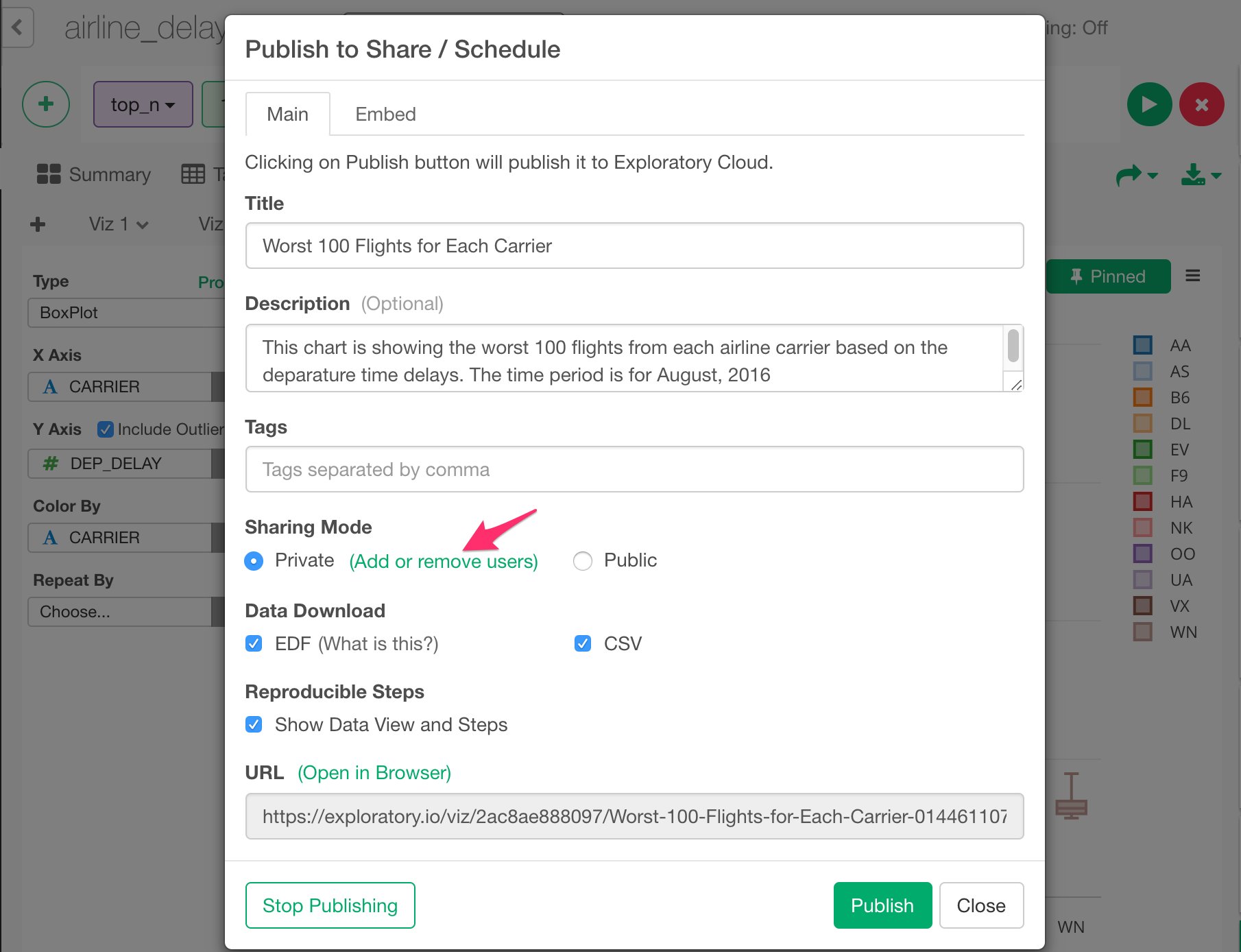
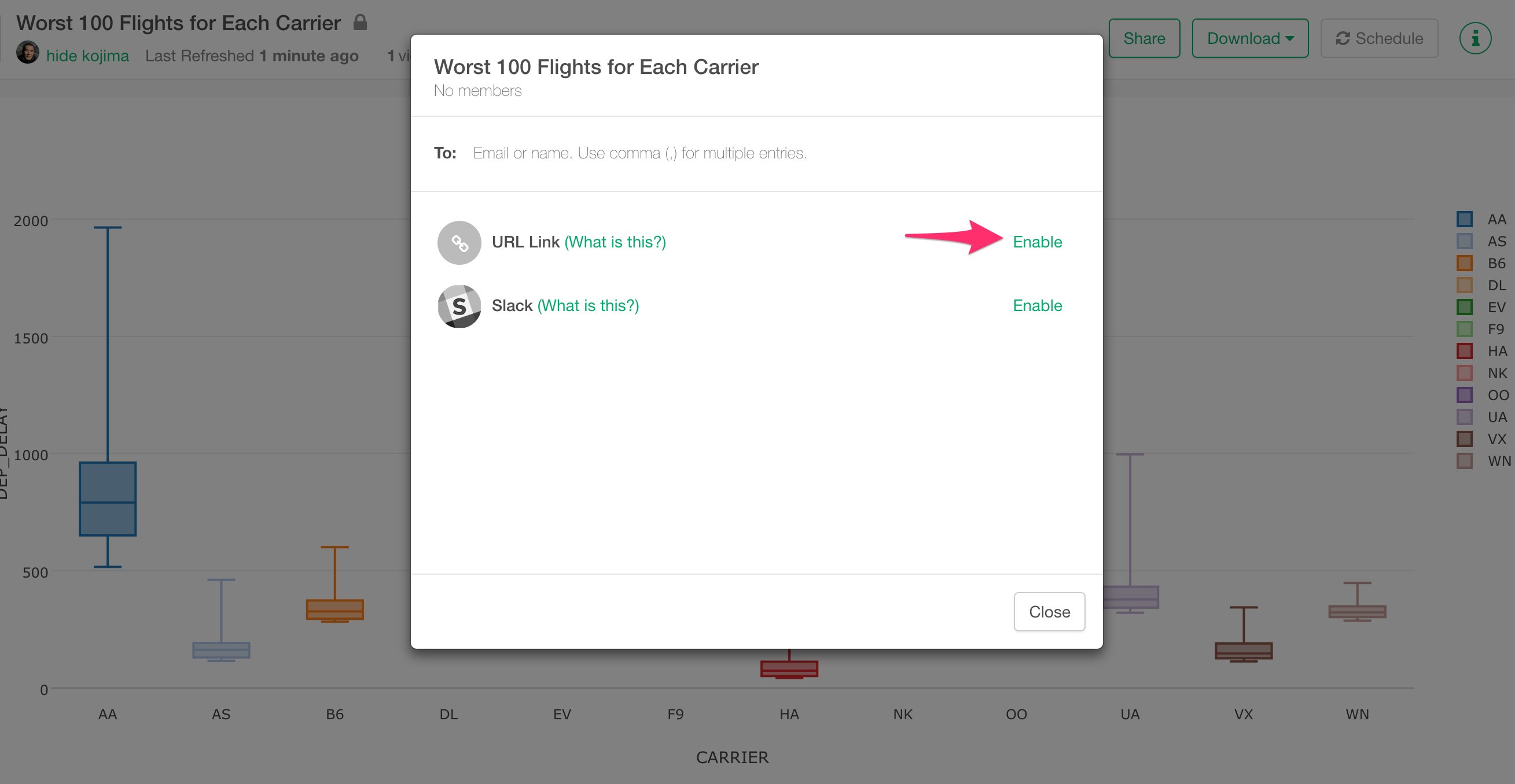
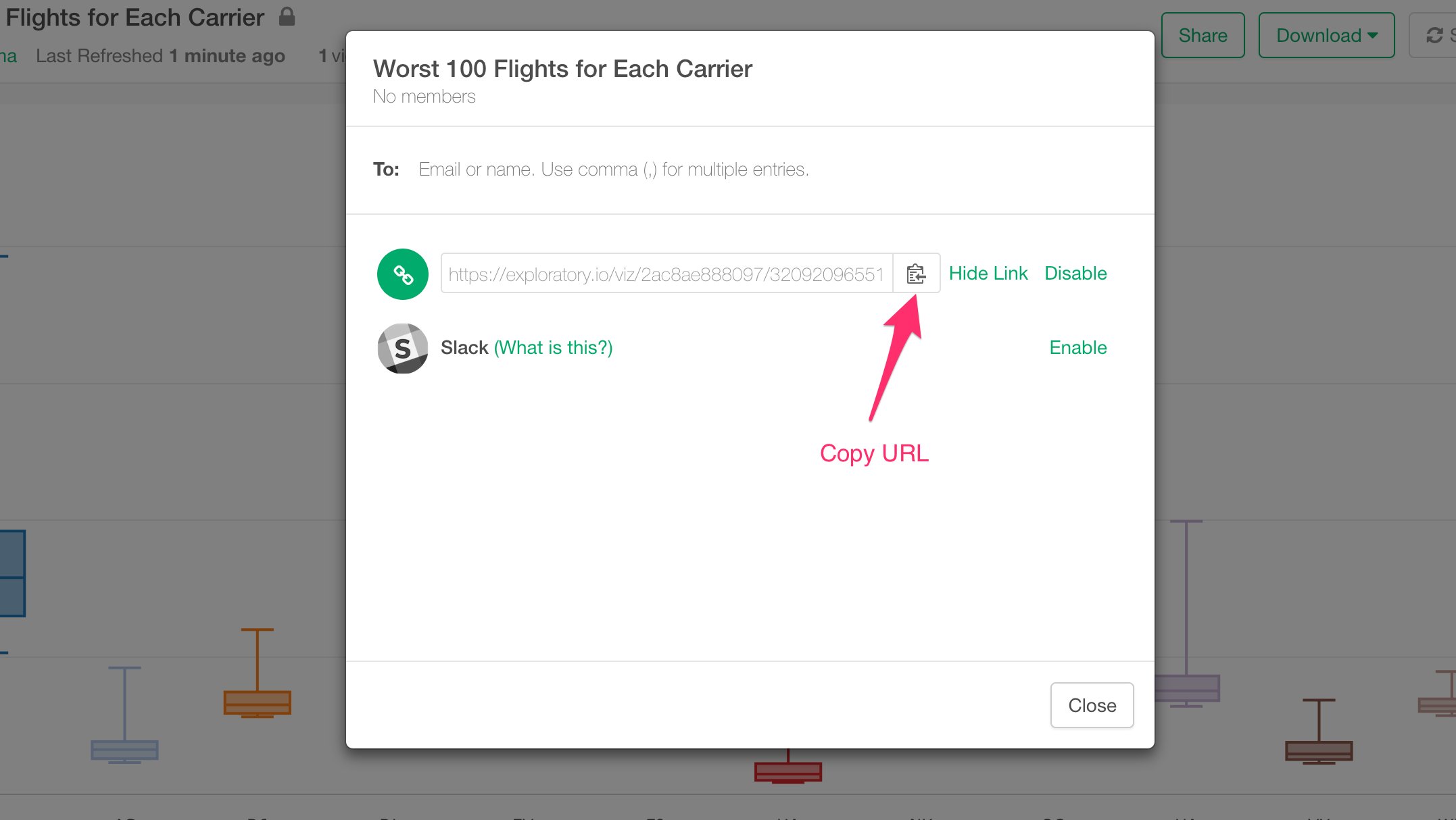
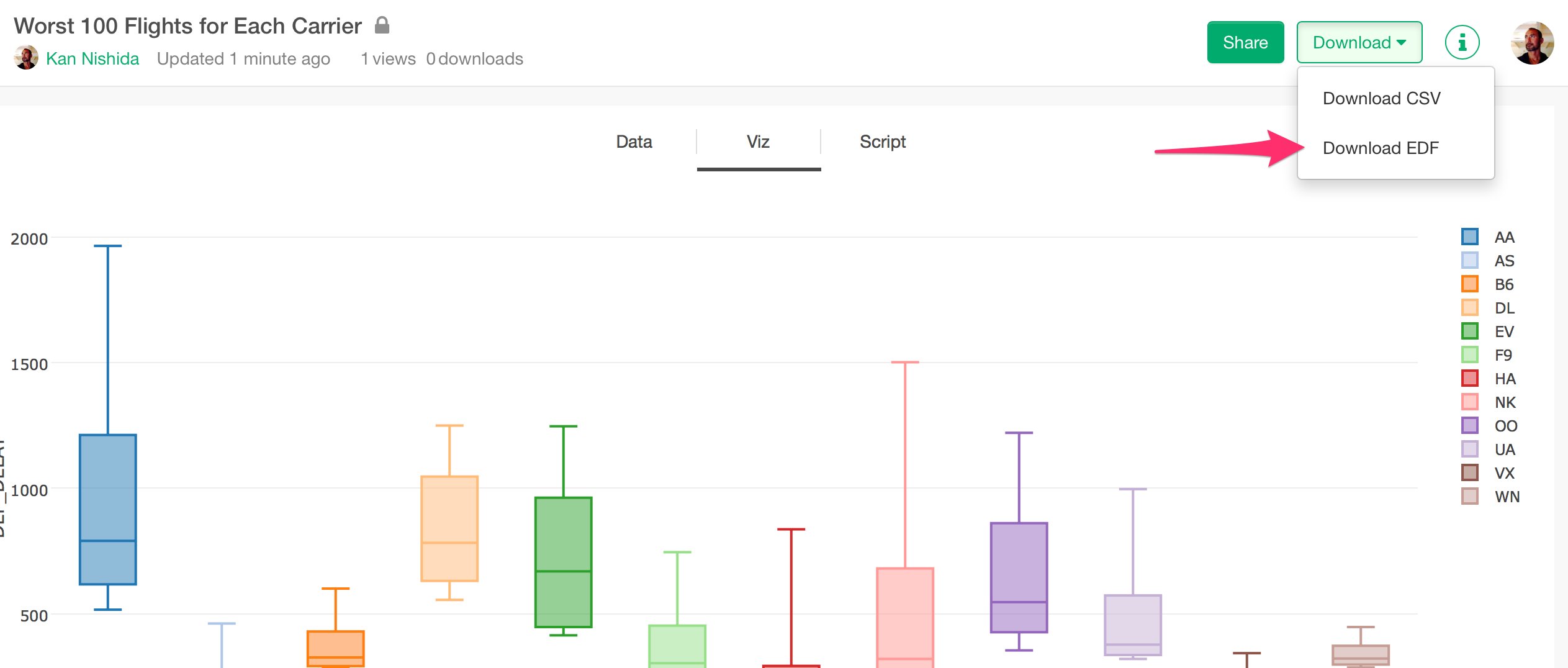
Once you find an interesting insight you might want to share it with others. With Exploratory, you can easily share not just the chart, but also the data wrangling steps along with the chart so that others will be able to reproduce your work easily. Select ‘Share Viz’ under ‘More’ button.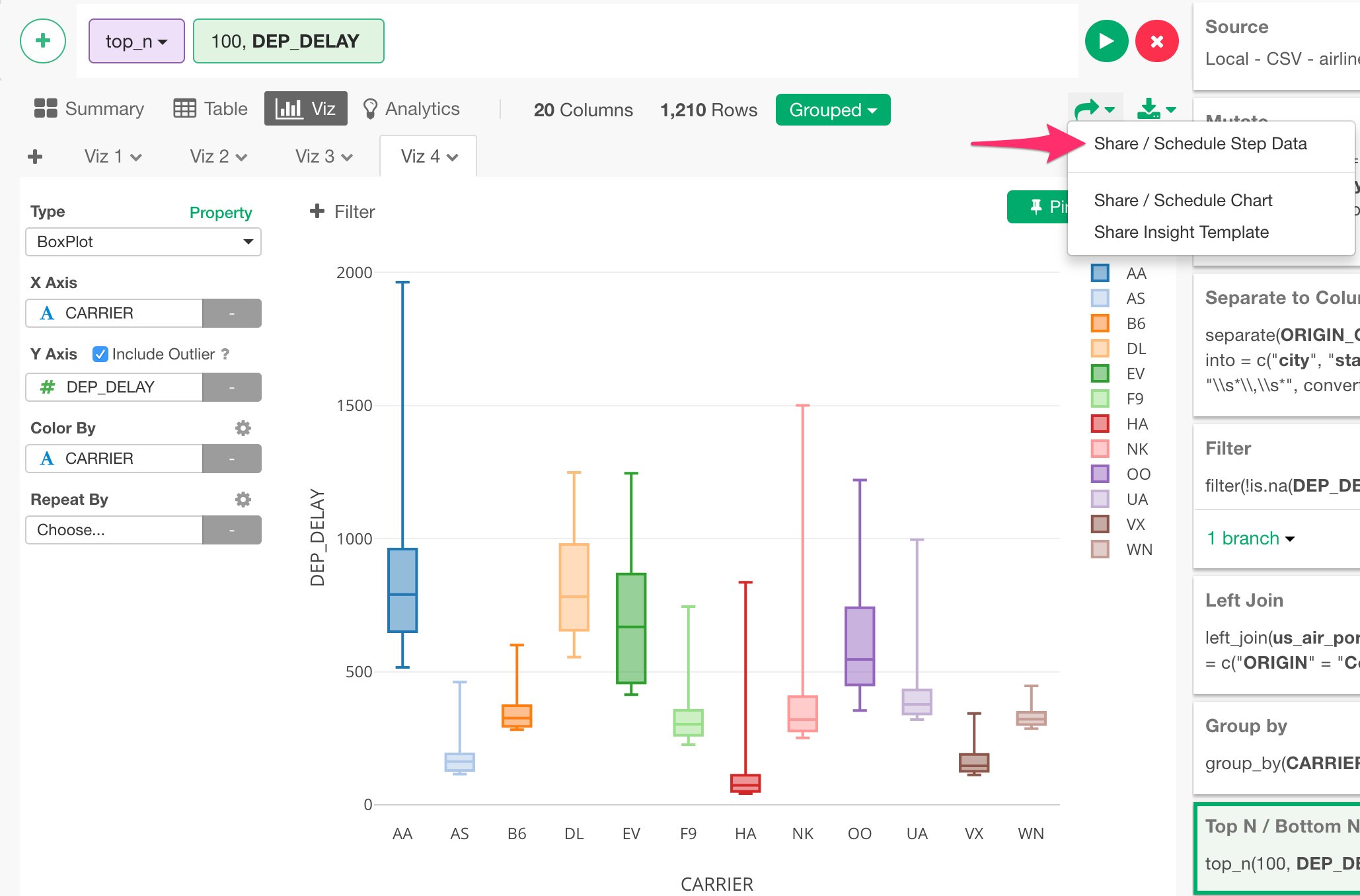
Create Note with Simple Markdown Editor
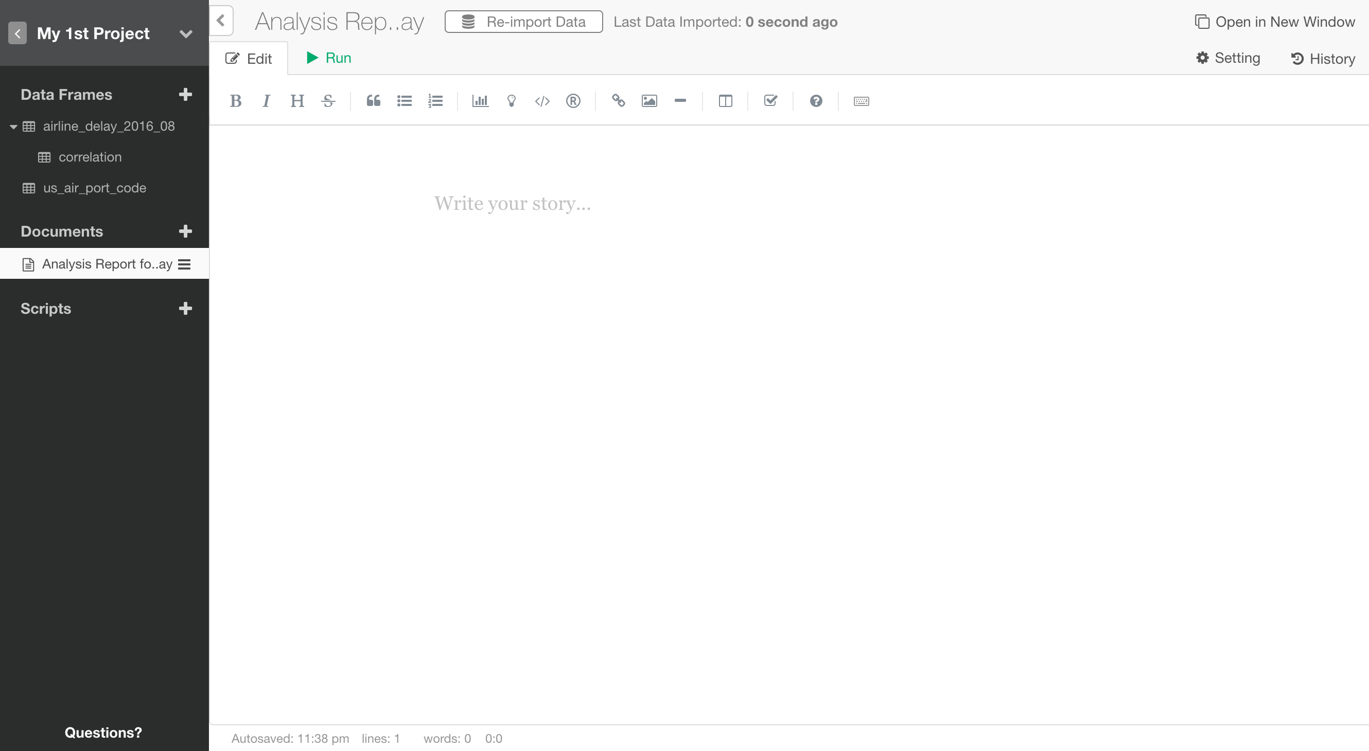
Once you find insights from your data analysis, you want to communicate it with others by authoring, publishing, and sharing Notes. In this section, let’s quickly take a look at how you can do such in Exploratory. Click ‘Plus’ button next to ‘Note’.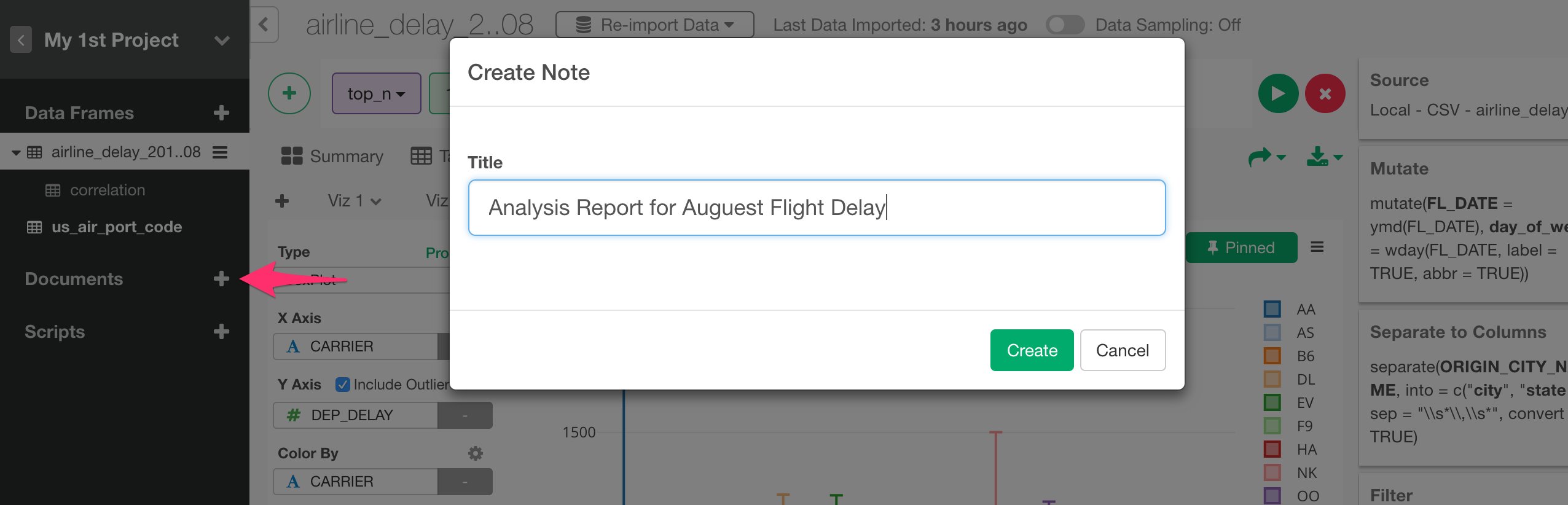
Preview the formatting output
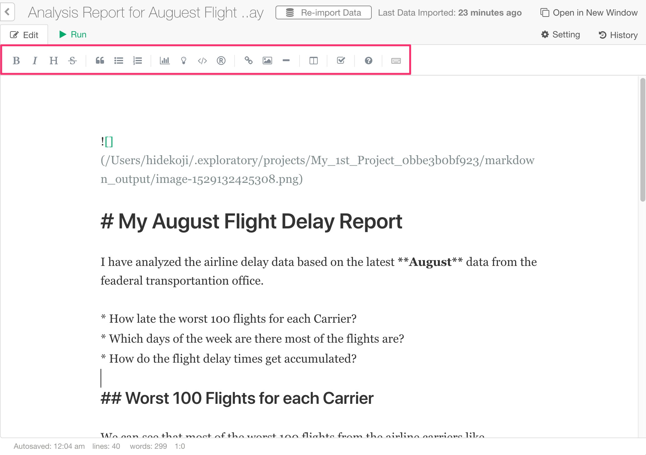
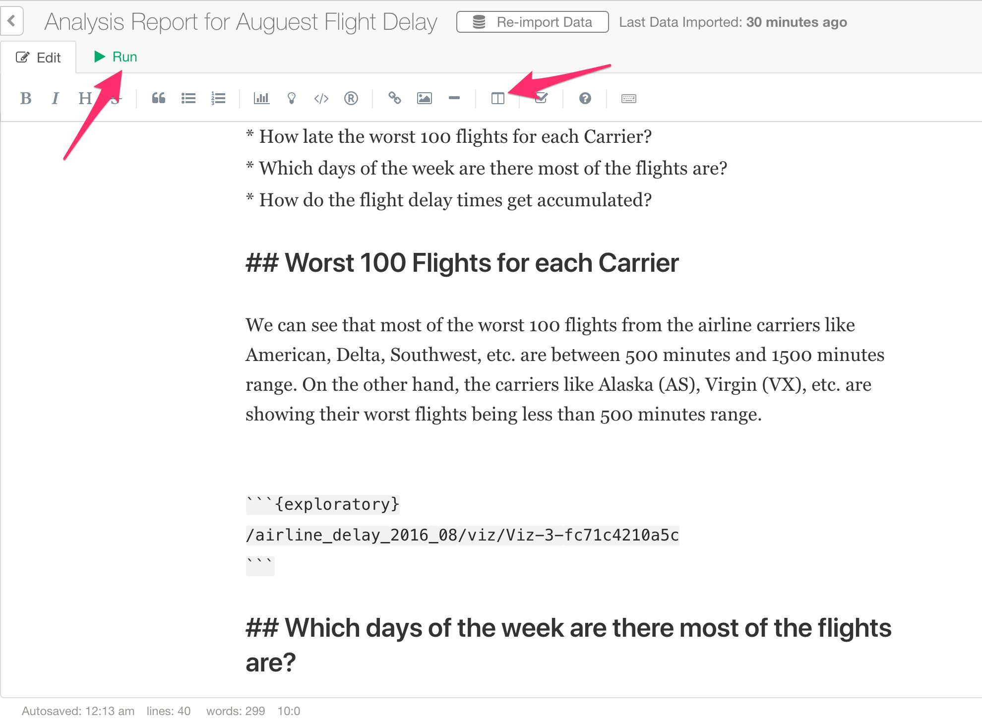
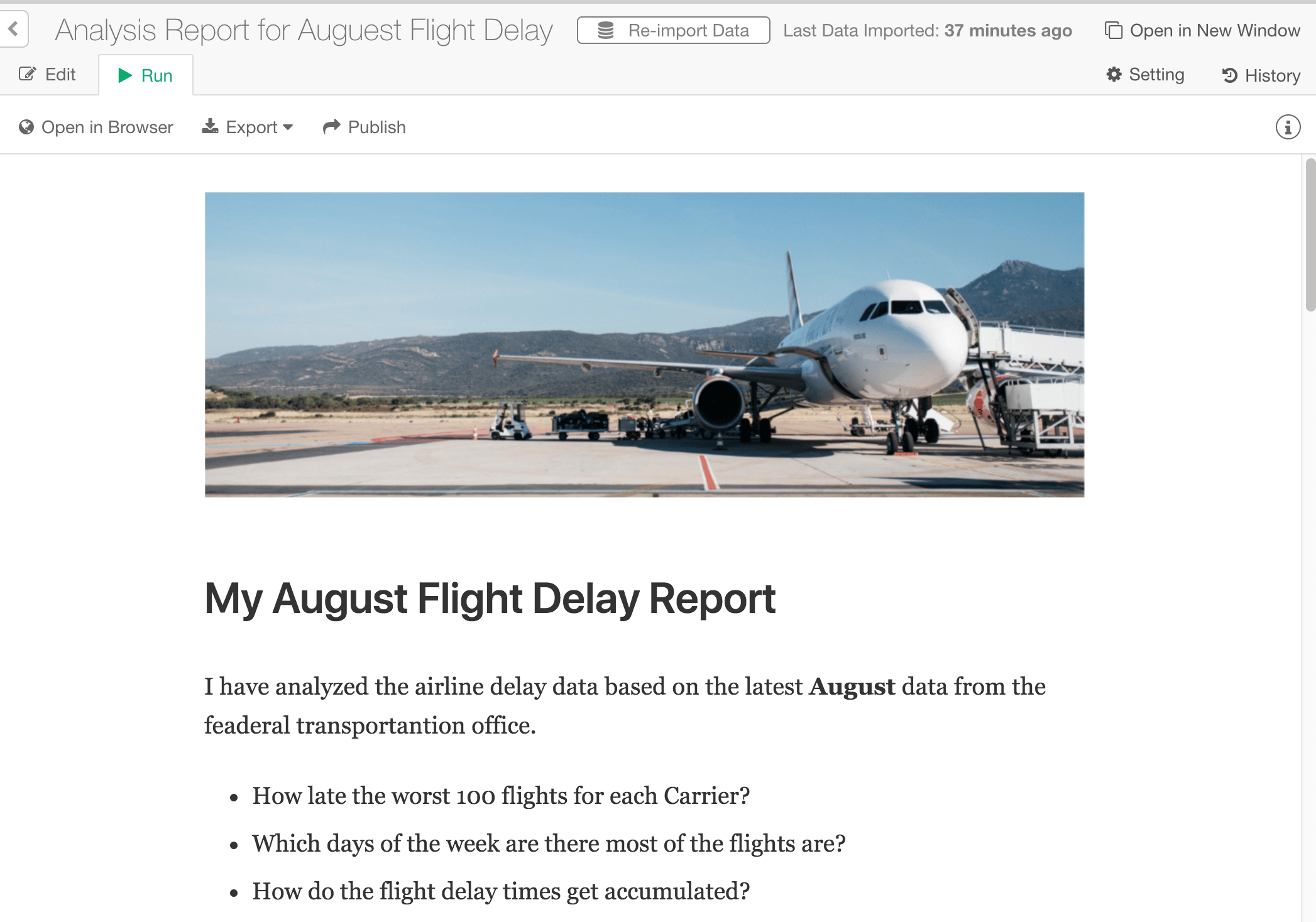
You can preview the markdown formatting (e.g. Header text, images, bullet points, etc.) style by clicking on one of the preview buttons in the toolbar.
Insert Charts from Visualization or Analytics View
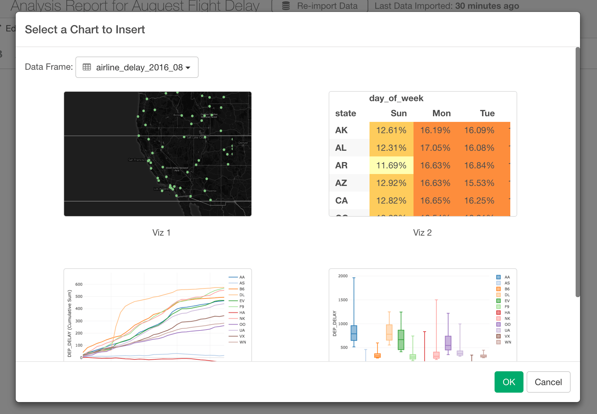
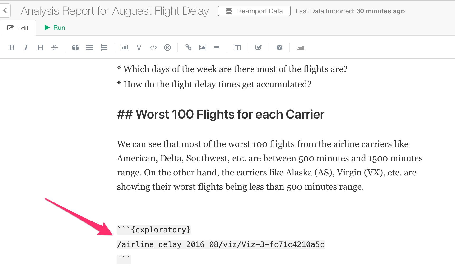
You can insert the charts you have created at the previous steps for the flight data by clicking on Chart icon in the toolbar.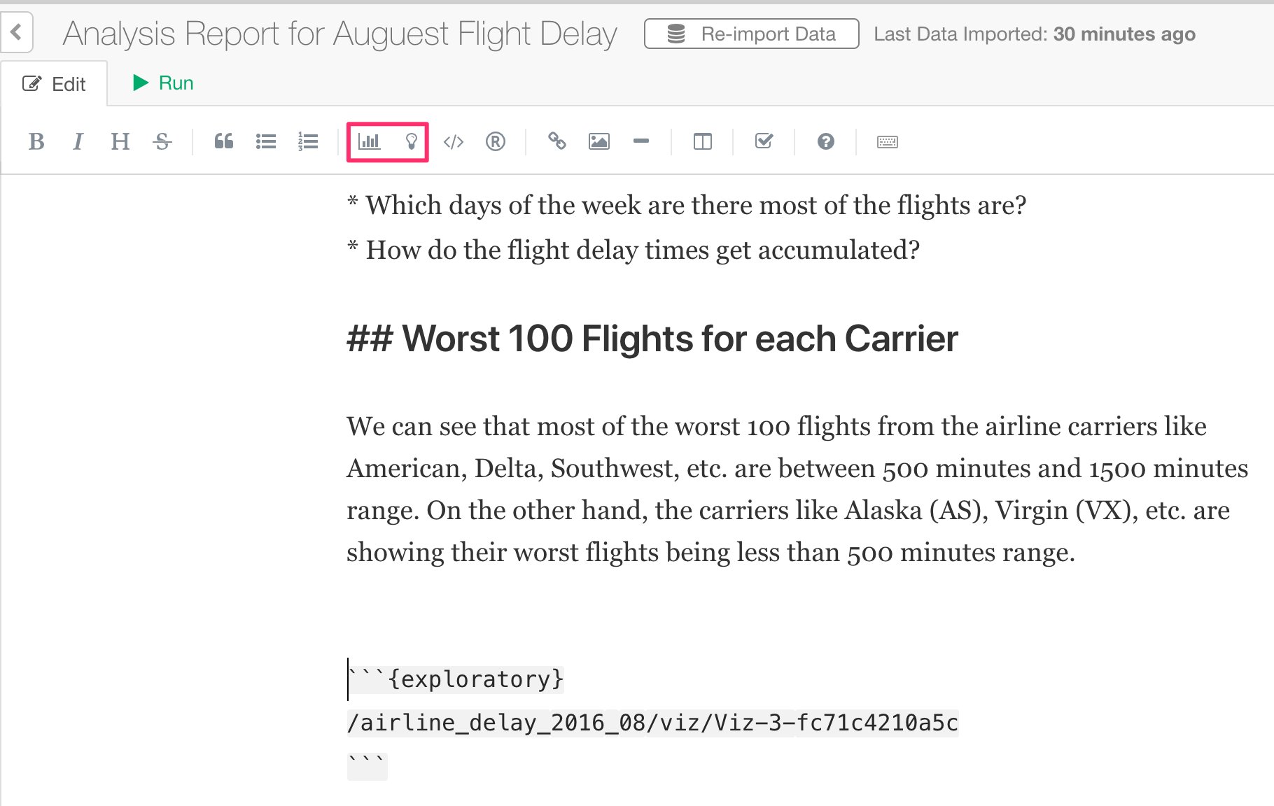
Insert R Code
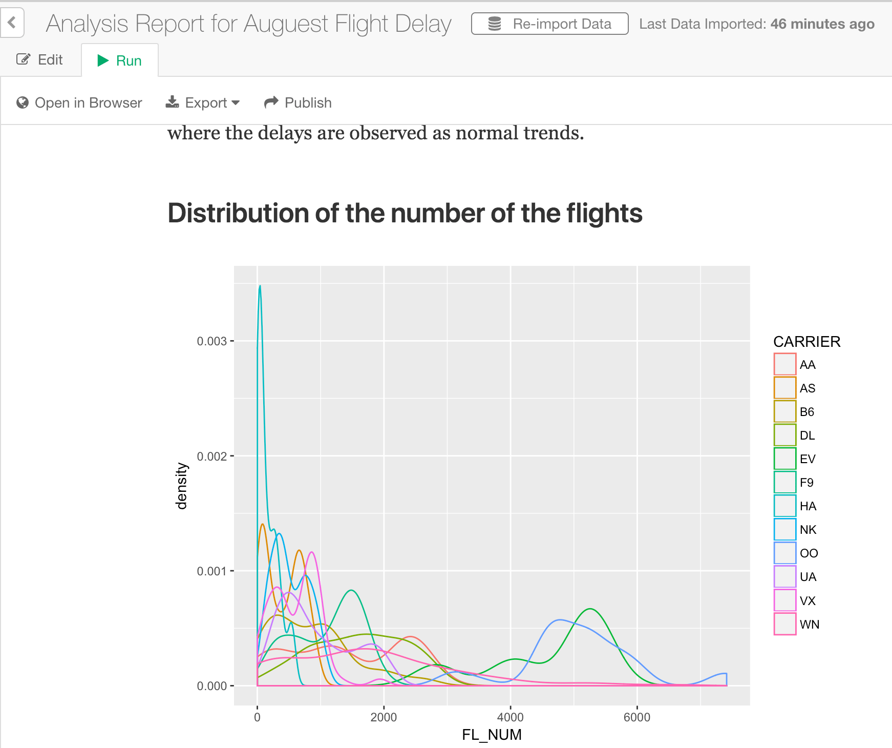
If you are familiar with R programming language, then you can write R script with your favorite R packages like ggplot2 to present your data as well.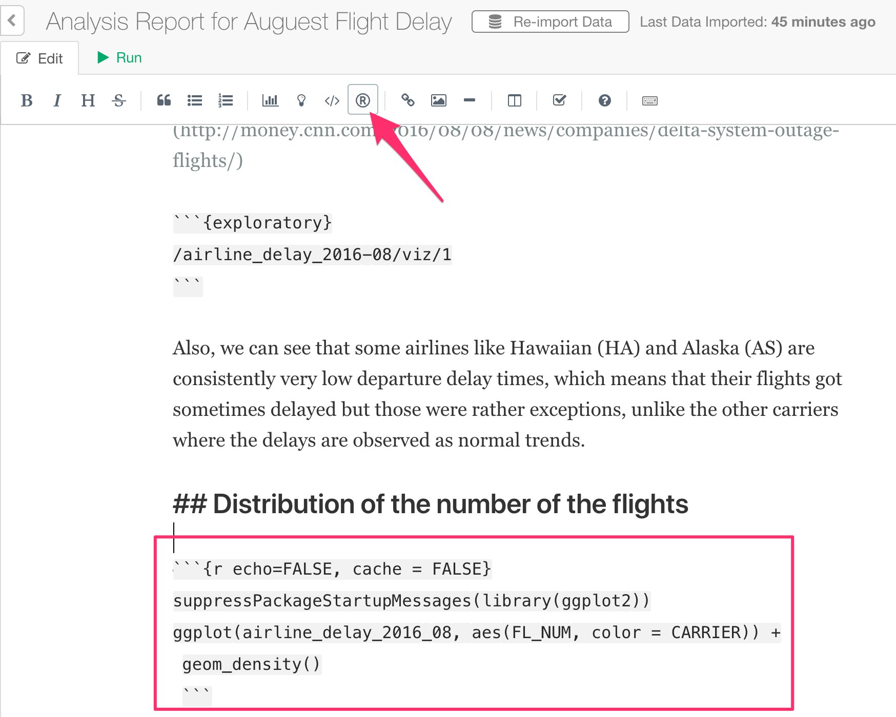
Congratulations! You have finished the tutorial. Now you know how to use Exploratory to start taking advantage of the latest and greatest of the technological advancements in Data Science and start finding much deeper insights from your data quickly! If you have any questions, feel free to contact Team Exploratory. Cheers! Team Exploratory